Sensitivity of radiative forcing to global carbonaceous emissions

1. Introduction

Both fossil fuel and biomass combustion, which are the principal sources of anthropogenic SO₂, generate direct emissions of carbonaceous aerosols of varying composition, ranging from elemental carbon to volatile organic compounds (VOCs). Organics are the largest single component of biomass burning aerosols (Andreae et al., 1988; Artaxo et al., 1988; Cachier et al., 1995) which can scatter as much light as sulphate (Charlson et al., 1991, 1992; Kiehl and Briegleb, 1993; Boucher and Anderson, 1995; Hegg et al., 1997); dust and black carbon (BC) on the other hand, can be effective radiative absorbers (Andreae, 2001; Satheesh and Srinivasan, 2002; Kim et al., 2006; Moorthy et al., 2007). A significant fraction of carbonaceous aerosols, especially the elemental carbon fraction is strongly light absorbing (Chylek et al., 1984; Penner et al., 1998; Cooke et al., 1999; Jacobson, 2000; Koch, 2001; Chung and Seinfeld, 2002). Further, radiation absorbing aerosol particles in the atmosphere, such as BC, have a significant influence on global climate. This discussion thus signifies that scattering and absorption of radiation by carbonaceous particles produce both direct and semidirect radiative forcing in the atmosphere.

Organic carbon (OC) is more rapidly scavenged from the atmosphere than BC (Cachier et al., 1991) that is why the latter component has larger atmospheric residence time than the former. The residence time of BC is believed to be equal to or longer than that of sulphate (Ogren and Charlson, 1984), which is about 5 d to a week. Interestingly, these aerosols have properties that range from light absorbing to light scattering in the atmosphere; a characterisation which essentially arises from their composition (Penner et al., 1993; Cooke and Wilson, 1996; Cooke et al., 1996; Bond et al., 2004) and, as a consequence, produce varying responses in the atmosphere depending on their distribution in the vertical as well. The presence of polar functional groups, particularly carboxylic and dicarboxylic acids, makes many of the organic compounds in aerosols water-soluble and allows them to participate in cloud droplet nucleation (Saxena et al., 1995; Saxena and Hildemann, 1996; Sempéré and Kawamura, 1996). Because the BC aerosols have a role to play in changing climate as suggested by the average radiative forcing calculated by Schulz et al. (2006), their concentration (especially of BC) should be accurately determined in atmospheric general circulation models (AGCMs). Moreover, BC particles may exist in the atmosphere as either insoluble particles, or in mixtures that are considered soluble. Hence, it will be efficiently removed from the atmosphere by dry deposition of insoluble BC particles and wet deposition of soluble mixtures of BC, thereby imparting it a shorter atmospheric residence time (Chylek et al., 1999; Hetzenberger et al., 2001; Zuberi et al., 2005). Thus, AGCMs must quantify the amount of BC that exists in insoluble versus soluble/mixed states. For simplicity, many AGCMs assume that surface based sources are comprised of BC emitted as 80% insoluble and 20% soluble parts, while OC emitted as 50% insoluble and 50% soluble parts (Cooke et al., 1999; Lohmann et al., 1999; Koch, 2001; Chung and Seinfeld, 2002; Cooke et al., 2002; Horowitz, 2006). In our study, we have assumed the same partitioning between soluble and insoluble parts of carbonaceous aerosols. Moreover, BC after its emission is subjected to several atmospheric processes, which include oxidation, condensation and coagulation. These processes, termed as the aging processes, act to change the solubility of BC aerosol. The aging of BC and organic matter (OM) is represented by a transfer of the hydrophobic to hydrophilic form with an exponential lifetime of 1.63 d (Reddy and Boucher, 2004; Reddy et al., 2005a).

Major sources for carbonaceous aerosols are biomass and fossil fuel burning, and the atmospheric oxidation of biogenic and anthropogenic VOCs. The global emission of organic aerosols from biomass and fossil fuel burning has been estimated at 45–80 Tg yr⁻¹ (Liousse et al., 1996; Cooke et al., 1999; Scholes and Andreae, 2000). Estimates of BC global emissions from biomass burning are in the range of 6–Tg yr⁻¹ (Penner et al., 1993; Cooke and Wilson, 1996; Liousse et al., 1996; Cooke et al., 1999; Ackerman et al., 2000; Scholes and Andreae, 2000; Koch, 2001; Chung and Seinfeld, 2002; Chin et al., 2002). The global BOND inventory yields a global BC burden of 8 and 33.9 Tg for OC, lower than the values of previous estimates (annual BC emissions of 7.96 Tg from fossil fuel combustion and 5.98 Tg from biomass burning) given by Cooke and Wilson (1996).

The major differences between the BC and OC inventories of Global Emission Inventory Activity (GEIA; Cooke et al., 1999; www.geiacenter.org) and of BOND arise mainly from the methodology of estimating their release in the atmosphere from emission factors that are used for fossil fuel combustion and biomass burning. While GEIA adopts a regional approach for estimating and improving further the emission factors, BOND inventory recognises the importance of technology in determining the emission factors, which depend on fuel type, activity sector and technology. Although there is associated uncertainty with each approach, nevertheless the technology weighted emission factors used in the BOND inventory provides the best estimate. GEIA emissions of BC and OC from fossil fuel sources are from Cooke et al. (1999); global emissions of BC for 1984 sum up to 6.4 Tg C yr⁻¹, while OC emissions of 10.1 Tg C yr⁻¹ were found using bulk aerosol emission factors. Global BC emissions of 5.1 Tg C yr⁻¹ and OC emissions of 7.0 Tg C yr⁻¹ were found using the submicron emission factors. The BC emissions from biomass burning are from Cooke and Wilson (1996); biomass burning emissions amount to 5.98 Tg yr⁻¹ and that from fossil fuel amounts to 7.96 Tg yr⁻¹. The OC emissions from all types of biomass burning sources are derived by assuming an OC to BC ratio of 7.0, which lies within the range used by Liousse et al. (1996) and Chin et al. (2002). We include in this study, secondary OC from terpene by assuming a conversion rate of 11% of terpene emissions from seasonal terpene emission distributions of Guenther et al. (1995). The conversion rate of 11% of terpene to produce secondary OC in the model is within the experimental range determined by Pandis et al. (1991) and results in natural OM emissions of 13.9 Tg yr⁻¹.

Bond et al. (2004) emissions of fossil fuel, biofuel and open burning are estimated as 38, 20 and 42%, respectively, for BC and 7, 19 and 74%, respectively, for OC (8.0 Tg yr⁻¹ for BC and 33.9 Tg yr⁻¹ for OC). These estimates are lower by 25–35% from previously published estimates. Since Bond et al. (2004) use measured BC fractions (1%) instead of guess values (25%) adopted by Cooke et al. (1999), there is a reduction in emissions for coal based power generation activity (difference 1.5 Tg yr⁻¹). The other sectors contributing to notable differences in emissions of these two inventories comprise sources from on-road diesel burning (difference 1.0 Tg yr⁻¹) and domestic diesel combustion (difference 0.25 Tg yr⁻¹).

How do these inventories compare with that of Horowitz (2006), which has been used for the Intergovernmental Panel on Climate Change (IPCC) 2007 Report? The key inputs for this report are Cooke et al. (1999) inventory for BC and OC, Hao and Liu (1994) estimates of biomass burning emissions in the tropics, and of Müller (1992) in the extratropics with emission ratios of Andreae and Merlet (2001). The biomass burning emissions are ‘climatological’ and do not vary from year to year and reflect that actual burning has occurred during specific years. Biogenic emissions of isoprene and monoterpenes are taken from GEIA (Guenther et al., 1995), with a 25% reduction in tropical isoprene emissions. Thus, the Horowitz (2006) do not use any emissions from the Bond et al. (2004) inventory. The main conclusion of Horowitz (2006) study with the Geophysical Fluid Dynamics Laboratory coupled climate model is that burdens of aerosols are sensitive to modelled rates of wet deposition.

In the present study, we simulate the atmospheric cycle of carbonaceous aerosols and estimate aerosol optical depth (AOD) using the GEIA and BOND inventories for primary BC and OC emissions. In an earlier study, De Meij et al. (2006) have evaluated AOD for EMEP and AeroCom inventories and found that AOD is less sensitive to the underlying emission inventories and show high spatial resemblance with satellite data. Here, we use the aerosol optical properties from Reddy and Boucher (2004) and Reddy et al. (2005a, b). BC is emitted only from combustion sources, but OC emissions include combustion as well as natural biogenic sources. We have analysed two carbonaceous emission inventories, viz. GEIA and BOND, from the response they respectively produce in a GCM. The GEIA inventory considers seasonal BC emission from biomass burning. OC emissions from all types of biomass burning sources with an aforementioned OC to BC ratio would introduce some uncertainty in the OC emissions from biomass burning sources as this ratio depends on biomass types. Hence, the magnitude and seasonality of emissions from open biomass burning would then also vary from year to year in different regions. Natural OC emissions include condensation of VOCs emitted from biogenic sources. Note that there is a very large uncertainty in global annual Secondary Organic Aerosol (SOA) production from biogenic sources because its estimates by Tsigaridis and Kanakidou (2003) range from 2.5 to 44.5 Tg OM yr⁻¹. Oxygen, hydrogen and other chemical species are always associated with OC, and the resulting aerosol is called OM. In this study, the OM to OC ratio of 1.4 and 1.6 has been used respectively for fossil fuel and biomass burning sources following the earlier studies of Turpin and Lim (2002), Reddy and Boucher (2004) and Reddy et al. (2005a). The BOND inventory considers the variability in different kinds burning of the same fuel as emission factors and aerosol type depend on burning conditions. The unique feature of the BOND inventory is that it provides full uncertainty propagation both regionally and sector-wise (Bond, 2005). For example, wood burning in domestic sector produces largest uncertainty (>25%) in BC and OC emissions in different part of the world. But for other sectors, uncertainty in BC emissions dominates over that in OC emissions (uncertainty >10%) even in the developed countries where it originates mainly in the usage of diesel.

2. Model description

The global atmospheric model used for this study is the standard general circulation model (Sadourny and Laval, 1984) of Laboratoire de Météorologie Dynamique (LMDZ version 3.3) coupled with interactive chemistry and aerosol dynamics as described in Verma et al. (2007). The global grid point LMDZ model with 19 vertical layers in hybrid sigma pressure coordinate and a horizontal resolution of 3.75° in longitude and 2.5° in latitude, includes a tropospheric chemistry module developed by Verma et al. (2007) and an aerosol module adapted from Model-3/CMAQ (Binkowski and Roselle, 2003) of US Environmental Protection Agency. The chemistry module includes anthropogenic and biogenic emissions; over 50 gas/aqueous phase chemical reactions (33 gas phase and 18 aqueous phase) along with the sources and sinks of chemical species are considered in this model. The sulphuric acid vapour produced from gas-phase chemistry drives the two-mode, two-moment aerosol module (Binkowski and Roselle, 2003) to calculate aerosol mass, number concentration and particle surface area for the Aitken and accumulation modes; while the sulphate from aqueous phase oxidation largely goes in the accumulation mode. The chemical species, aerosol mass and number concentration in the two modes are advected in the model and evolve consistently with dynamical, physical, cloud and chemical processes as model integration advances in time.

The prognostic chemical species in the LMDZ model are water vapour, liquid water, dimethylsulphide (DMS), hydrogensulphide (H₂S), dimethylsulphoxide (DMSO), methanesulphonic acid (MSA), sulphur dioxide (SO₂), oxides of nitrogen (NOx), carbon monoxide (CO), ozone (O₃), hydrogen peroxide (H₂O₂) and sulphate aerosol mass and number for Aitken (0.005–0.1 µm) and accumulation modes (0.1–2.5 µm). To account for the effect of clouds in the grid box, the clear sky photolytic rates are multiplied by a correction factor. Since a major part of atmospheric sulphate is produced in the clouds, aqueous-phase reactions are an integral part of the chemistry module. The aqueous-phase chemistry considers oxidation of SO₂ by O₃ and H₂O₂ only in the cloudy portion of the grid cell and in the presence of liquid water. During computations SO₂, H₂O₂ and O₃ concentrations in cloud droplets are regarded in equilibrium with the gas-phase concentration and are computed as a function of gas-phase concentrations. As regards scavenging in the model, both in-cloud and below-cloud scavenging have been considered. The CO₂ concentration is held constant (370 ppm) throughout the model integration.

3. Design of experiments

Numerical simulation experiments have been carried out using a complex atmospheric circulation model including chemistry and aerosol physics schemes and two emission inventories primarily to analyse the differences between the two inventories by examining aerosol burden, AOD and radiative forcing. The key hypothesis for these experiments is that aerosols are considered externally mixed and the conclusion of this study should therefore be viewed in the light of this assumption. The LMDZ.3.3 model at 96×72×19 resolution has been used to perform 5-year simulation runs with initial conditions that have been prepared from the 12 GMT ECMWF analysis of 20 December 1997. The sea-surface temperature (SST) fields were prescribed from the daily NCEP optimally interpolated SST data available from its ftp site (ftp://eclipse.ncdc.noaa.gov/pub/OI-Weeky/NetCDF). The surface albedo, soil moisture, snowlines and sea-ice were prescribed from climatology. The optical properties of each individual aerosol species have been calculated by shutting off other aerosols in respective simulations.

Depending upon their chemical nature, carbonaceous aerosols take up water and grow in size with increasing RH. We consider this RH effect on particle size for the hydrophilic OM following Tang and Munkelwitz (1994) and Tang (1997). The refractive index for the hydrophilic aerosols at a given RH is computed as a volume weighted average of the respective aerosol and water refractive indices. We use the model's clear-sky RH with a maximum value at 95% as far as aerosol growth factor f(RH) is concerned and use tabulated values of f(RH). The ambient humidity corrected particle size is then used for calculating the optical parameters in the model for performing radiative transfer computations. In each numerical experiment, the initial 1-year simulation is referred to as the model spin-up period; and the subsequent 4-year simulation run outputs were analysed to obtain the results and to arrive at the conclusions of this study.

4. Results and discussions

The main difference between two emission inventories (Cooke et al., 1999; Bond et al., 2004) is that the inventory of Cooke et al. (1999) is based on a guess value of BC (25%) instead of measured BC fraction (<1%) used by Bond et al. (2004). The latter inventory used measured emissions and World Bank data instead of assuming that developing countries have five times higher emissions as in the former. Also, Bond et al. (2004) do not use emissions factors for internal combustion engines to external combustion boilers that affect the emissions over Europe.

Two sets of independent model simulation runs of 5-year duration, have been performed by prescribing emissions form each inventory. The simulated aerosol burdens, AODs have been analysed and compared with other models (AeroCom-median, CAM, GOCART and GISS) in order to assess how these quantities evolved in the annual mean in simulations with LMDZ. AeroCom-median is the median of the response of the participant models in the ‘Aerosol module inter-Comparison in global models (AeroCom) initiative’ as aerosol modules in global models require initial assessment before being used for constructing future scenarios of climate variations. The AeroCom has been the first such assessment that documented the differences from aerosol component modules in global models (Kinne et al., 2006; Schulz et al., 2006; Textor et al., 2007. The simulations were performed for AeroCom by constraining the participant models with a prescribed set of global natural and anthropogenic emissions for the year 2000 from one of the best inventories compiled by Dentener et al. (2006) that was available in the year 2003, viz., the AeroCom inventory (ftp://ftp.ei.jrc.it/pub/Aerocom). The 15 monthly varying large scale biomass burning emissions of Particulate Organic Matter (POM), BC and SO₂ are based on Global Fire Emissions Database 2000 as described by Van der Werf et al. (2003). Fossil fuel/biofuel related POM (47.0 Tg POM yr⁻¹) and BC (8.0 Tg C yr⁻¹) emissions are based on Bond et al. (2004). AeroCom assumes that 15% of natural terpene emissions are form SOA altogether amounting to 19.11 Tg POM yr⁻¹. The simulations may therefore be assessed if their outputs are evaluated with the results of some participant models of AeroCom.

The impact of the differences between two inventories could be evaluated more precisely by evaluating the response of the model with the help of a normalised difference (ND), which is essentially an index such that − 1 < ND < 1. This index may be defined for any quantity A, which is a function of some prognostic variable in the model. We define the ND of the quantity A as:

1

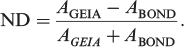
where the quantity A may represent aerosol burden, optical depth or any other model variable. If ND<0, then the higher values of quantity A are simulated by the model with BOND inventory, while on the contrary; ND > 0 will imply that superior values of the quantity A are simulated with GEIA inventory in comparison to those simulated by the model with BOND inventory. However, if ND ~ 0 with both A _GEIA>0 and A _BOND>0, the values of A are nearly same over a particular region in the model simulations with both inventories. Thus, the ND-plots would provide a fairly clear comparison of the two inventories from model responses that they produce in long-term simulations. We have evaluated for this study the NDs of aerosol burden, AOD, and direct radiating forcing of the carbonaceous aerosols at the top of the atmosphere (TOA), which have greatly facilitated the analysis in identifying important differences in the two inventories. These quantities have also been compared with simulated fields of some of the AeroCom models by downloading them from the site: http://dataipsl.ipsl.jussieu.fr/AEROCOM/aerocomhome.html.

4.1. Aerosol burden

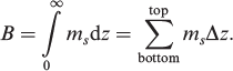
Atmospheric aerosols are ubiquitous, but their horizontal and vertical distributions in the atmosphere are highly variable. Since the opacity of the atmospheric column directly depends on the aerosol loading in the vertical, therefore aerosol burden, that is the vertically integrated mass of an aerosol species, is one of the key elements that need to be analysed while comparing different inventories. The burden (B) is defined as the product of the mass of the species (m _s ) in an atmospheric layer and the layer depth (dz) summed up over all the model layers. Thus, the column burden (mg/m²) has been computed as follows:

2

4.1.1. BC aerosols burden.

The BC aerosols global annual mean burden is estimated to be 0.17 Tg BC (GEIA) which matches with the estimate of Chen et al. (2010). A further observation is that our estimate falls within the range of 0.15–0.25 Tg BC given by Cooke et al. (1999) and it is also closer to the estimate (0.19 Tg BC) of Reddy et al. (2005a). The global annual mean burden estimated with the BOND inventory is 0.07 Tg BC. The distribution of annual averages of the BC burden (Fig. 1a) suggests that a strong model response with GEIA inventory is seen over equatorial Africa. The model simulations with both inventories (Fig. 1a and b) also suggest the presence of pristine air beyond 60°S. A distinct feature of the simulation with the BOND inventory is that the region of pristine air over Greenland is comparatively of larger expanse than that is simulated with the GEIA inventory. The LMDZ simulated BC burdens are also compared with the median (Fig. 1c) of AeroCom participant models, and simulations of GISS (Fig. 1d), GOCART (Fig. 1e) and CAM (Fig. 1f) models that were constrained by prescribing with emissions from the AeroCom inventory (Dentener et al., 2006).

Fig. 1. 

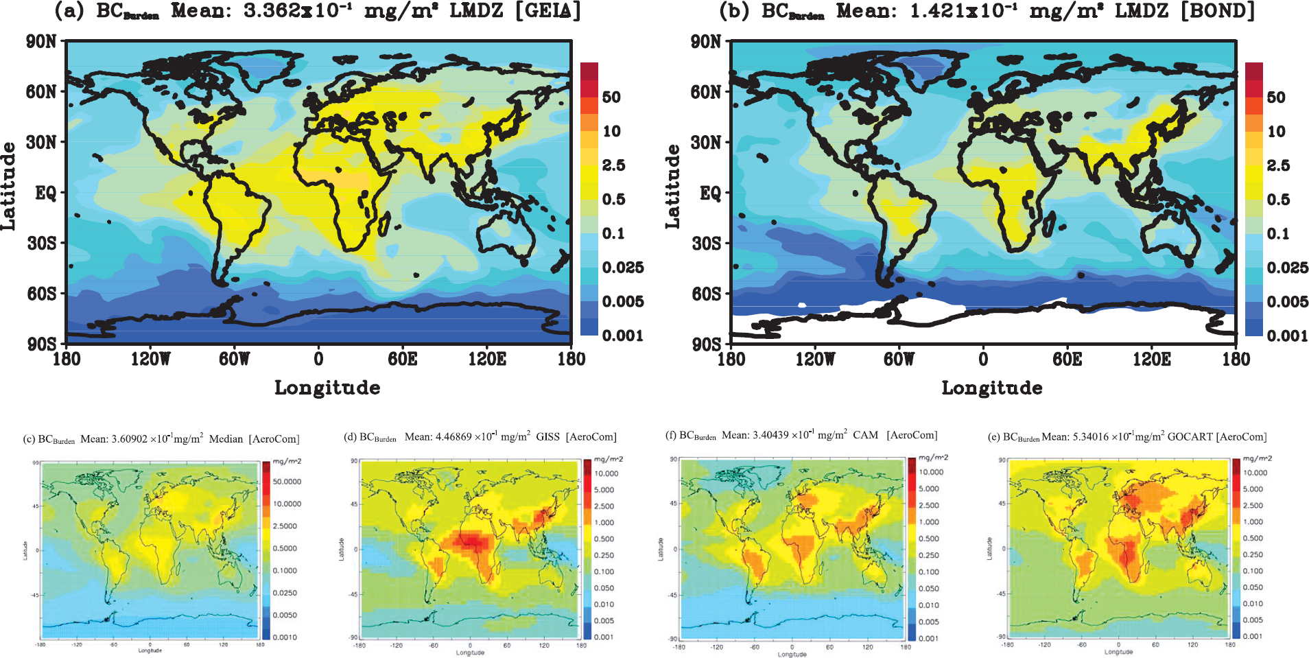
The BC aerosol burdens simulated by LMDZ with GEIA and BOND inventories show a striking similarity in spatial distribution with those of AeroCom-median (Fig. 1c) and CAM simulated (Fig. 1f) BC burden distribution though the simulated burdens with BOND inventory are relatively smaller in magnitudes over some parts of the globe. A visual inspection of different panels in Fig. 1 shows that while BOND burden (1.421×10⁻¹ g m⁻²; Fig. 1b) is comparatively of smaller magnitude to GEIA burden (3.363×10⁻¹ g m⁻²; Fig. 1a), but the latter agrees very closely with AeroCom burden (3.609×10⁻¹ g m⁻²; Fig. 1c) and the CAM simulated BC burden (3.404×10⁻¹ g m⁻²; Fig. 1f). Also, BC burden values as simulated in the present study are systematically lower over the Australian region in comparison to the corresponding AeroCom and CAM values. From the above comparison of BC burdens, it may be said that the distribution LMDZ model simulated BC burden with GEIA and BOND inventories shows closer agreement with the corresponding AeroCom and CAM distributions than that of GOCART and GISS simulated burdens though GISS simulation uses BOND emissions. Hence, the model simulations show lower BC burdens for BOND inventory and closer agreement with GEIA inventory when compared with AeroCom BC values (Schulz et al., 2006; Koch et al., 2009).

4.1.2. OM aerosols burden.

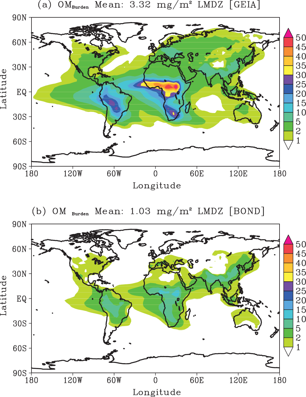
For OM aerosols (Fig. 2), the global annual mean burden simulated in this study with GEIA inventory is 1.66 Tg OM, which is comparatively lower than the estimated burden (1.75 Tg OM) of Reddy et al. (2005a) but exceeds the value of the burden (1.10 Tg OM) reported by Chen et al. (2010). However, with the BOND inventory, LMDZ simulates global annual mean burden as 0.5 Tg OM, which is significantly lower than the above-mentioned estimated burden of OM with GEIA. Higher burdens of OM over South Africa and South America regions (Fig. 2a and b) are simulated, in particular, with the GEIA inventory.

Fig. 2. 

4.1.3. Mixed carbonaceous aerosols burden.

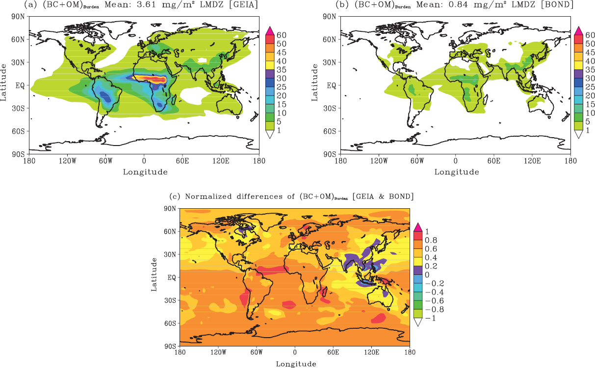
Annual global average of carbonaceous aerosols has been simulated by LMDZ as 106.0 and 38.0 Tg yr⁻¹, respectively for GEIA and BOND inventories. Central estimates (between low and high values) of global annual emissions are 8.0 Tg for BC and 33.9 Tg for OC (Bond et al., 2004). The LMDZ simulates higher burden of carbonaceous aerosols (Fig. 3a) over equatorial and southern Africa and South America with GEIA emissions in comparison to those of BOND (Fig. 3b), which is mainly due to forest fires in these regions (Schultz et al., 2008). The NDs of carbonaceous aerosol burden simulated with two inventories – GEIA and BOND – show that they are closer over northeastern India, Bangladesh, Indo-China region, northern Pacific, and Australia (Fig. 3c), but show large differences over rest of the globe. Also, one may observe from Fig. 3c that a large amount of carbonaceous aerosols are transported over the Tropical Atlantic Ocean with higher burdens in the equatorial region. Thus, the meteorology plays an important role in the long range transport of the carbonaceous aerosols over the oceans from southern and Equatorial Africa.

Fig. 3. 

4.2. Aerosol optical depth

AODs link the atmospheric aerosol loadings to their radiative effects. AOD is a measure of transparency, which is related to extinction by the aerosol components in the atmosphere. AODs typically decrease with increasing wavelength. It is expressed for any species as the product of mass extinction efficiency, mass of the species and the layer depth; that is:

Mathematically, the above relation is expressed as:

3

The radiative transfer code in the LMDZ consists of improved versions of parameterisations of Fouquart and Bonnel (1980) for solar radiation and Morcrette (1991) for terrestrial radiation. The optical properties (mass extinction efficiency α _e , single-scattering albedo ω, and asymmetry factor g, are obtained from Mie theory by using a lognormal size distribution and refractive indices (Boucher and Anderson, 1995; Köpke et al., 1997; O'Dowd et al., 1997; Guelle et al., 2000) which have been given for the dry aerosol in Table 1 at the wavelength 550 nm. In the radiative transfer code of LMDZ, the shortwave spectrum is divided into two wavebands: 0.25–0.68 and 0.68–4 µm; optical properties are computed over the entire shortwave spectrum (0.25–4 µm) at 24 wavelengths and grouped into the two model wavebands as weighted averages with a typical spectral distribution of the incoming solar radiation flux at the surface. AODs have been computed with the help of optical parameters given in Table 1. The function f(RH) depends on humidity and allows aerosol growth or swelling of particles in humid environment. In our model, we have used a look-up table to efficiently compute the growth of the aerosol particles due to humidity. The AOD at 550 nm in this study for the BC aerosols has been also compared with those of the other models (Fig. 4) in order to assess its distribution and magnitude in different parts of the globe.

Fig. 4. 

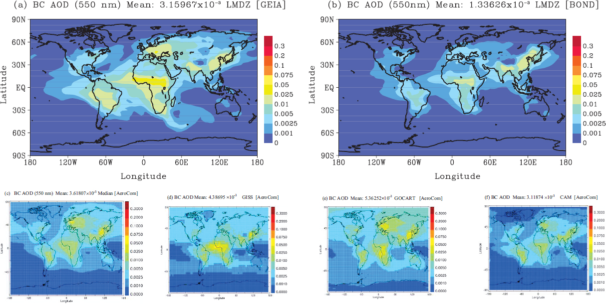
Table 1. Physical and optical properties at (550 nm) of dry aerosol (BC and OM)

Aerosol type Dry density (ρ) (g cm⁻³) Modal radius (r₀) (µm) Geometric SD (σ_g) Refractive index Mass extinction coefficient (α_e) (m² g⁻¹) Single scattering albedo (ω) Asymmetry factor (g) BC 1.0 0.0118 2.0 1.75–0.45i 9.412 0.21 0.34 OM 1.8 0.0355 2.0 1.53–0.005i 3.159 0.97 0.61

4.2.1. AOD (550 nm) of BC aerosols.

Higher AOD levels for BC aerosols have been simulated in the Northern Hemisphere over Europe, in the Southern Hemisphere over South Africa and South America with GEIA inventory. The simulated AOD in other parts of the globe with the two inventories show greater agreement and differ in the range of ±20% only. AOD is directly proportional to mass concentration of each species. Annual average of AOD (550 nm) of BC aerosols has been plotted in Fig. 4a and b for GEIA and BOND inventories.

AOD (550 nm) simulated with BC aerosols is different for these two emissions inventories over South Africa, South America and Europe. However, results from both inventories match fairly well over India and China (Fig. 4a and b) suggesting that in these regions, despite the obvious differences in emissions in the two inventories (noted also in their respective burdens in Fig. 1). The dispersal of BC aerosol horizontally and vertically by the simulated meteorology of the region could be responsible for this sort of matching in the model response despite the divergences in emissions (Textor et al., 2007; Koch et al., 2009).

Since computation of AOD uses BC burdens hence the spatial distribution of AOD will closely follow the BC burden distributions as may be seen in Fig. 4a and b. Accordingly, AOD fields from GEIA inventory agree closely in magnitudes with that of AeroCom (Fig. 4c) and CAM (Fig. 4f) simulated AODs. As expected, AOD simulated by LMDZ with BOND (Fig. 4b) inventory is relatively smaller in magnitude than that with GEIA (Fig. 4a), so also with those of AeroCom (Fig. 4c) and CAM (Fig. 4f) simulated fields. The main defect in the simulations of AODs with LMDZ may be noted over the Australian region where AODs (Fig. 4a and b) are too small in comparison those of the median AOD levels and CAM simulated AODs with AeroCom inventory. This comparison shows that model simulations reproduce correct distribution of AOD over most parts of the globe. The mean value of 3.15967×10⁻³ of simulated AOD with GEIA inventory (Fig. 4a) is closer to the median value 3.6180×10⁻³ of AOD (Fig. 4c) of models that have been constrained by prescribing emissions from AeroCom inventory. The model simulated AOD mean value of 1.33626×10⁻³ with BOND inventory (Fig. 4b) is relatively smaller in magnitude. It may therefore be inferred that the LMDZ simulated correctly AODs both in magnitude and distribution for BC aerosols, and values are fairly in good agreement with the AODs reported in the intercomparison study of AeroCom models (Table 3 of Schulz et al., 2006).

4.2.2. AOD (550 nm) of OM aerosols.

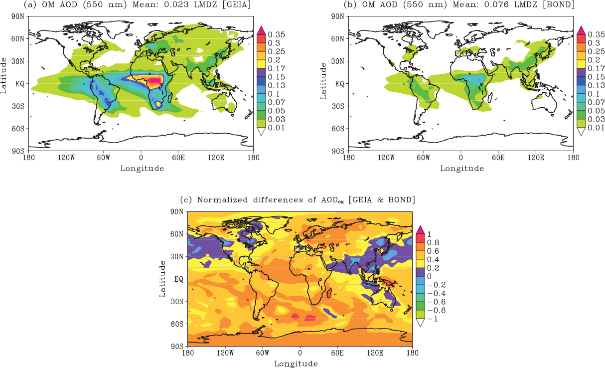
The annual averages of AOD (550 nm) for OM aerosols have been plotted in Fig. 5a and b. It could be observed from this Fig. 5, that mostly, GEIA emissions produce elevated levels of AOD in comparison with that from BOND emissions. But if we plot the NDs (Fig. 5c), then it has been observed that BOND OM emissions have produced higher response in AOD over northeast India, some parts of China, and from the effect of transport of the OM over some part of North Pacific Ocean (30–60 N) may also be noted in this Fig. 5c.

Fig. 5. 

4.2.3. AOD (550 nm) of carbonaceous aerosols.

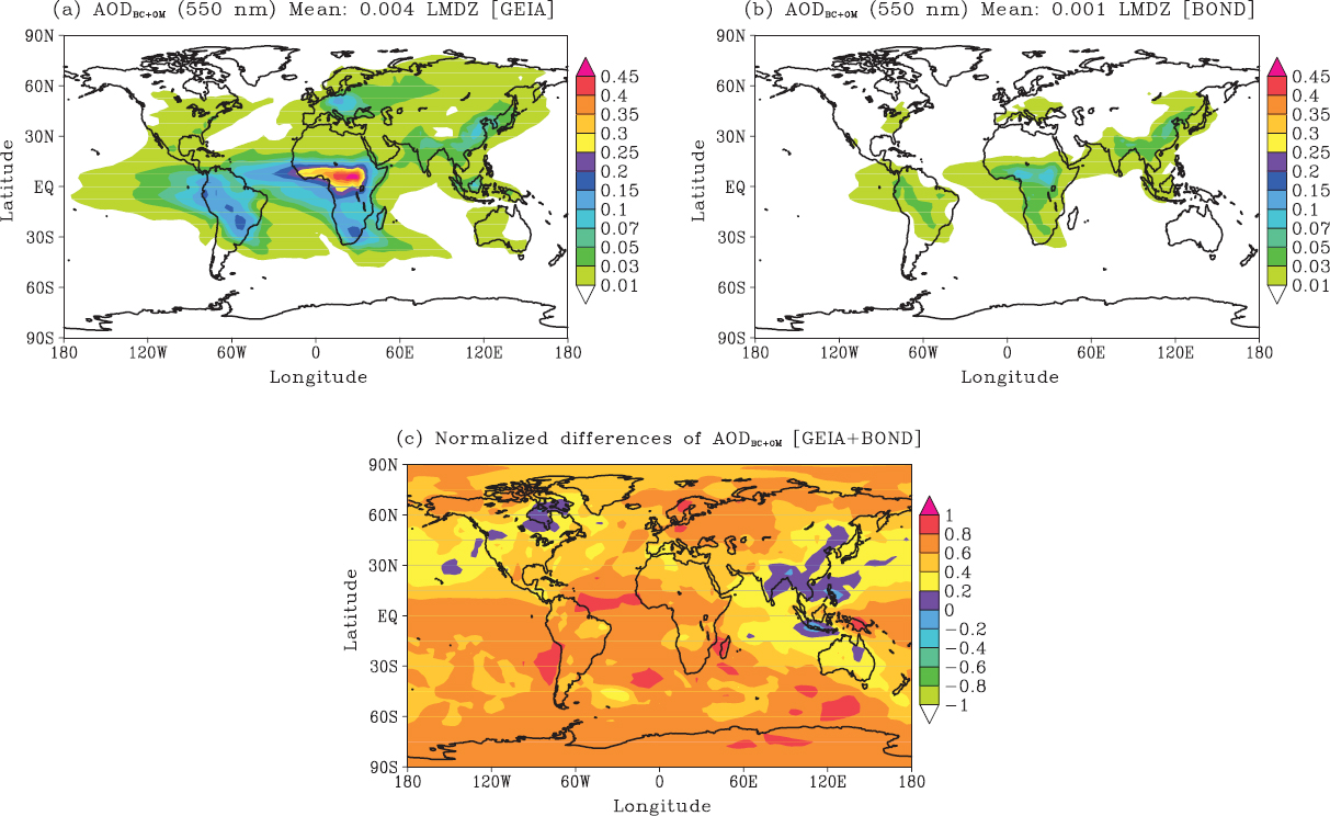
A similar inference is derived from the plots of simulated global annual average of AOD of carbonaceous aerosols (BC + OM) as shown in Fig. 6a and b. It is worth pointing out that the response of the model from different inventories is better seen in the NDs of simulated quantities such the aerosol burdens, which distinctly portrays the differences in corresponding simulations. The comparison of NDs shows that model simulates higher response globally with GEIA inventory except over Jakarta and Philippines (Fig. 6c).

Fig. 6. 

4.2.4. DRF at the TOA.

Direct radiative forcing (DRF) is computed as the difference between the shortwave fluxes (SWFs) at the TOA without aerosol loading (SWF₀) and with the aerosols included (SWF _a ) in the numerical simulations. Direct effect refers to the direct scattering or absorption of radiation by aerosol particles without any modification of cloud properties. From the optical characteristics (optical depth, single scattering albedo, asymmetry parameter, etc.) of the aerosols, their size distributions, and changes due to relative humidity effects, the radiative fluxes can be computed as:

4

4.2.5. DRF (TOA) of BC aerosols.

BC plays a major role in the surface and TOA forcing (Penner et al., 1992; Hansen et al., 1997; Haywood and Shine, 1997; Podgorny et al., 2000; Schultz et al., 2006; Koch et al., 2009). BC aerosols absorb solar radiation and produce positive radiative forcing at the TOA (Fig. 7a and b) in LMDZ simulations. Over South Africa and South America and some part of Europe, the radiative forcing is observed to be more due to GEIA emissions than the BOND emissions. BC emissions give positive radiative forcing at TOA and negative at the surface because of solar dimming. The effect is predicted to be considerable in regions of high BC concentrations such as Africa, South America, Northern Europe, China and India (Fig. 7a and b). Normalised differences of TOA DRF of BC aerosols show that it is simulated higher in magnitudes everywhere with GEIA emissions except northeast part of India, northern part of Australia and Jakarta. Their influence dominates over Europe and some parts of Russia, Madagascar, South Atlantic Ocean and the Arctic Ocean (Fig. 7c).

Fig. 7. 

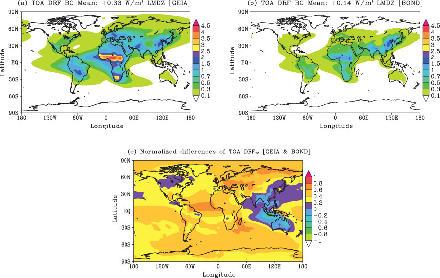
The BC radiative forcing is positive with a global average value of +0.25 Wm⁻² for the AeroCom models (Schultz et al., 2006). In comparison to this value, the BC radiative forcing simulated by the LMDZ model is +0.33 and +0.14 W m⁻², respectively, with GEIA and BOND inventories. A comparison of direct TOA radiative forcing for BC has been given in Table 1. The TOA forcing of +0.33 W m⁻² (GEIA) of BC aerosols is quite closer to the values given by Koch (2001), Haywood et al. (1997) and Jacobson (2001) as shown in Table 2. The smaller radiative forcing in Jacobson (2001) may have resulted due to the aerosols being modelled as tri-modal with lesser aerosol in the optically active region of the spectrum, or if absorption by BC were enhanced in the modelled multi-component mixture. The direct BC radiative forcing from LMDZ with GEIA and BOND inventories is comparatively much smaller to +0.9W m⁻² – a value obtained by Ramanathan and Carmichael (2008) that is based on observationally constrained study of Chung et al. (2005). In this context, an important question arises: Is this difference due to inventory, transport or radiative transfer model, or none of these? While Ramanathan and Carmichael (2008) attribute several reasons for the smaller direct BC radiative forcing in GCMs, but neglecting internal mixing of aerosols during computations and model simulated higher BC concentrations near the surface are the key responsible factors for lower direct BC forcing in models. Both of these factors could be responsible for smaller direct BC radiative forcing in this study due to the following reasons. Firstly, the aerosols are externally mixed in this study; hence, the direct BC radiative forcing is expectedly underestimated (by about a factor of 2) if the aerosols were internally mixed. Secondly, we have examined the zonally averaged burden of BC as simulated in LMDZ (figures not shown) and it is found that the concentrations are higher in the lower layers closer to surface, whereas it generally peaks at about 2 km (800 hPa) above the surface in observations. Such a distribution of BC would also produce lower TOA forcing as pointed out by Ramanathan and Carmichael (2008). Despite these limitations, our results compare fairly well with the estimates (0.2–0.4 W m⁻²) given by other general circulation models (Highwood and Kinnersley, 2006; IPCC, 2007; Koch et al., 2007). It may therefore be inferred that the difference between globally averaged direct BC radiative forcing simulated by LMDZ and of Ramanathan and Carmichael (2008) appears to be due to above factors and may not be due to inventory, transport or the radiative transfer model.

Table 2. Comparison of predicted DRF of BC aerosols with other estimates (W m⁻²)

Reference Emissions Mixing scenario Anthropogenic forcing (W m⁻²) This work FF and BB External +0.33 (GEIA) +0.14 (BOND) IPCC (2007) (anthropogenic emissions) FF +0.2 (±0.15) BB +0.03 AeroCom models Schulz et al. (2006) FF and BB (AeroCom emissions) +0.25 Chung and Seinfeld (2002) FF and BB (Cooke et al., 1999) External +0.51 Koch (2001) FF and BB (IPCC, 2000; Liousse et al., 1996; Penner et al., 1993) External +0.35 Jacobson (2001) FF and BB (Cooke External +0.27 and Wilson, 1996; Liousse et al., 1996) Internal +0.55 Haywood et al. (1997) FF and BB External +0.40

[i] FF = fossil fuel; BB = biomass burning.

4.2.6. DRF (TOA) of OM aerosols.

The annual average of TOA DRF due to OM has been plotted in Fig. 8 for GEIA and BOND emissions. In this figure the TOA forcing due to GEIA emissions is higher over southern Africa and South America in comparison to that from BOND emission inventory. The morphology of the model response over these continents (Africa and South America) is nearly same but they differ largely in their magnitudes. Normalised differences of the response of the model from GEIA and BOND OM emissions have been plotted in Fig. 8c, which suggest that in BOND emissions constrained simulations, the model response in TOA DRF is smaller in magnitude as compared to that with GEIA emissions over most of the areas on the globe except northeast India and North Pacific Ocean (30–60 °N).

Fig. 8. 

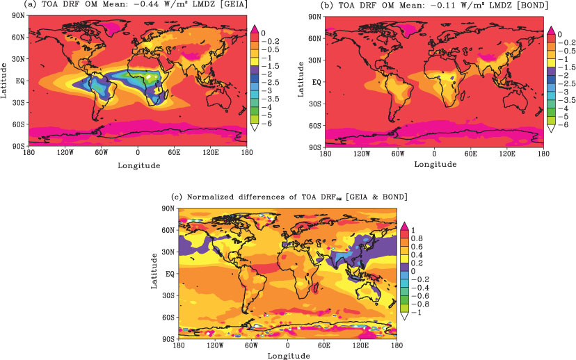
The annual radiative forcing due to OM from GEIA emissions has been calculated in the LMDZ as –0.44 W m⁻² whereas for the BOND inventory it is simulated as −0.11 W m⁻². The modelled DRF of OM aerosols has been compared in Table 3 with the previous estimates. The model-simulated estimates for DRF with GEIA inventory come out to be very close to those of Hansen et al. (1998) results, but much lower than that of Cooke et al. 1999 because it has considered only fossil fuel emissions. The smaller magnitude of DRF in Jacobson (2001) may have resulted due to internal mixing of aerosols. However, our estimate lies in the range given by IPCC (2007) from anthropogenic emissions.

Table 3. Comparison of predicted DRF of OM aerosols with other estimates (W m⁻²)

References Emissions Mixing scenario Anthropogenic forcing This work FF and BB External −0.44 (GEIA) −0.11 (BOND) Hansen et al. (1998) FF and BB External −0.41 Cooke et al. (1999) FF External −0.02 Jacobson (2001) FF and BB (Cooke External −0.057 and Wilson, 1996; Liousse et al., 1996) Internal −0.04 to − 0.06 AeroCom models Schulz et al. (2006) FF and BB (AeroCom emissions) −0.14 IPCC 2007 (anthropogenic emissions) FF −0.05 (±0.05) BB −0.2 range ~( 0.07 to − 0.6)

[i] FF = fossil fuel; BB = biomass burning.

4.2.7. DRF (TOA) of mixed carbonaceous aerosols.

The two emission inventories produce different responses in LMDZ in simulated radiative forcing of BC and OM aerosols considered together as carbonaceous aerosols. It gives a clear distinction between positive and negative forcing areas, mainly positive forcing in the Northern Hemisphere and negative forcing in the Southern Hemisphere (Fig. 9a). With BOND inventory, over South America and South Africa, there is relatively greater spread of positive forcing than the negative forcing (Fig. 9b). This type of distribution in forcing with BOND inventory suggests that BC aerosols are spread over larger areas in these regions. This contrast in simulations is also seen in the annual average of TOA radiative forcing for total carbonaceous aerosols with −0.014 W m⁻² (GEIA) and +0.118 W m⁻² (BOND). The net radiative forcing of carbonaceous aerosols with GEIA emissions is negative, but it is of opposite sign with the BOND emission inventory. The key point that emerges from these simulations is that the TOA radiative forcing appears to be highly sensitive to carbonaceous content in aerosol compositions.

Fig. 9. 

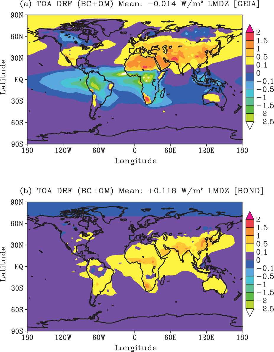
The carbonaceous aerosol budget calculated from the two inventories has been presented in Table 4. For GEIA emissions, BC emissions are by a factor of ~2 higher and OM emissions are also higher by about a factor of ~3 than the emissions in the BOND inventory. The burden due to BC and OM aerosols has the same ratio as their respective emissions. The DRF at TOA due to BC aerosols with GEIA (+0.33 W m⁻²) is ~3 times higher (Table 1) than BOND emissions (+0.14 W m⁻²). OM aerosols in GEIA inventory are four times higher than the BOND emissions (Table 2). Therefore the DRF of mixed carbonaceous aerosols have net negative ( 0.014 W m⁻²) forcing with GEIA emissions and net positive (+0.118 W m⁻²) forcing with BOND emissions. The forcing simulated with GEIA inventory shows closer agreement with other models (AeroCom and CAM).

Table 4. Comparison of emissions between GEIA and BOND inventories

GEIA Bond et al. (2004) Emissions, BC Tg yr⁻¹ 11 5 Emissions, OM Tg yr⁻¹ 95 33 Emissions, BC + OM Tg yr⁻¹ 106 38 Wet deposition, BC + OM Tg yr⁻¹ 77 26 Dry deposition, BC + OM Tg yr⁻¹ 29 12 Burden, BC Tg yr⁻¹ 0.17 0.07 Burden, OM Tg yr⁻¹ 1.66 0.5

The model calculated DRF might be interpreted as the change in radiative forcing arising from variations in the reflectivity of the aerosol layer enveloping the globe. If S ₀ (1370 W m⁻²) represents the Solar constant, then DRF may be equated to Δα _p S ₀/4 with Δα _p as the net change in the globally averaged planetary albedo and S ₀/4 as the global mean incident solar radiation flux at the top of the scattering aerosol layer. However, reflectivity will be reduced by an effective factor depending upon the single scattering albedo (w ₀) of the absorbing aerosols. Thus, we may write the globally averaged change in reflectivity (Δα _p ) for the atmosphere as a layer with absorbing aerosols as:

5

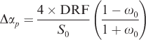
For a perfectly scattering layer: ω ₀=1 gives Δα _p =0, i.e. the change in reflectivity due to absorbing layer would vanish. The key advantage offered by eq. (5) is that it allows a direct comparison of different inventories of absorbing aerosols from their global responses in changing the albedo of the absorbing aerosol layer as it evolves during the model simulations. However, for this formula to be useful for practical applications, it is necessary that the values of Δα _p obtained from eq. (5), should be consistent with such calculations from the other formula used by Penner et al. (2001) for the IPCC (2001) Report, which has been originally proposed by Chylek and Wong (1995). The change in global average planetary albedo (IPCC, 2001, The Scientific Basis, p. 322) associated with anthropogenic aerosols is described as:

6

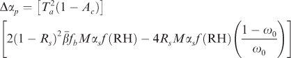
where,

T_a=atmospheric transmissivity above the main aerosol layer

A _c =global cloud fraction

R _s =global average surface albedo

=upscatter fraction for isotropic incoming radiation

f _b =hygroscopic growth factor for upscatter fraction

M=global mean column burden for aerosol constituent, (gm⁻²)

α _s =aerosol mass scattering efficiency, (m² g⁻¹)

f(RH)=hygroscopic growth factor for total particle scattering

w ₀=single scattering albedo at ambient RH (assumed to be 80%)

We can now compute Δα _p from formulae given by eqs. (5) and (6) for comparing the two inventories from model simulations. The change in globally averaged planetary albedo computed from eq. (5) for GEIA and BOND inventories are given by:

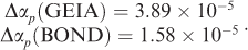
while corresponding values of Δα _p computed using eq. (6) of the IPCC (2001) Report are:

It may be noted that values of Δα _p computed from eq. (5) show only slight deviations from the corresponding values of Δα _{p_ipcc} obtained from eq. (6). For this reason, eq. (5) appears to be very appropriate for comparing different inventories from their response in model simulated DRF. Although the burden of BC aerosols with GEIA inventory is simulated almost twice of the amount with BOND inventory, yet the change that it produces in planetary albedo is ~2.5 times than that of the later. This shows that the impact of the burden is not linear on planetary albedo in model simulations.

4.3. Surface radiative forcing of carbonaceous aerosols

Surface radiative forcing is the difference between SWFs at the surface with and without the consideration of aerosols in the simulations. At the surface, radiative forcing is negative due to the solar dimming effect of aerosols. The key differences in the surface radiating forcing simulated with the two inventories considered here are seen mainly over South Africa, South America and Europe (Fig. 10a and b). However, over India and China surface radiative forcing is same from both the emissions inventories.

Fig. 10. 

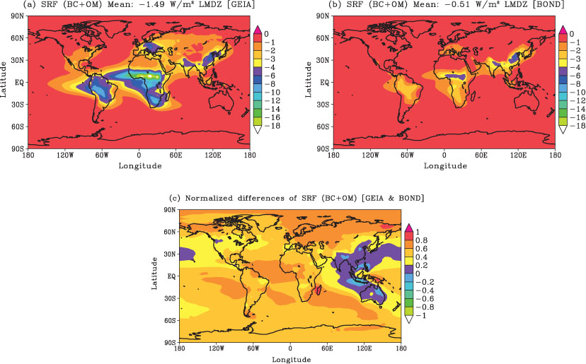
Annual average of surface radiative forcing is calculated as −1.49 W m⁻² (GEIA) and −0.51 W m⁻² (BOND), respectively, by the LMDZ model. The annual average surface radiative forcing calculated from AeroCom models is −1.02±0.23 (Schulz et al., 2006). Normalised differences of surface radiative forcing have been plotted in Fig. 10c, which are positive everywhere over the globe except over an arch-shaped region that extends from Pacific to parts of eastern China to eastern Australia with northeast India, Vietnam, some parts of Indonesia falling under this arch. That is, the model response in surface radiative forcing with BOND inventory exceeds only in these regions in comparison to that with the GEIA inventory. The LMDZ model in some parts of the Pacific has also simulated negative values in normalised surface radiative forcing differences with lowest values over Jakarta.

5. Conclusions

Annual global burden, AOD and radiative forcing of two carbonaceous emissions inventories have been compared. Annual global averages of burden of BC show that GEIA inventory induced burden in numerical simulations is approximately twice of that is simulated with the BOND inventory. However, the burden of organic aerosols simulated by the model is nearly three times of that with BOND inventory. The model produces higher AODs with GEIA over the entire globe except the Asian region and some parts of Australia. This is also true for the DRF of BC aerosols. But for OM aerosols, GEIA emissions calculate lower DRF only over the northeastern region of India in comparison to the BOND inventory. Mixed carbonaceous aerosols show clear distinction between positive and negative forcing areas because of dominance of BC and OM aerosols. Annual average of TOA radiative forcing for total carbonaceous aerosols is −0.014 W m⁻² (GEIA) and +0.118 W m⁻² (BOND). Annual average of surface radiative forcing is calculated as −1.49 W m⁻² (GEIA) and −0.51 W m⁻² (BOND), respectively. GEIA inventory produces more SRF than BOND inventory except over some parts in the Asian region and Australia.

TOA DRF of the BC aerosols in model simulations with the two inventories are +0.33 W m⁻² (GEIA) and +0.14 W m⁻² (Bond et al., 2004), respectively. On the contrary, for OM aerosols, TOA DRF is of opposite sign with −0.44 W m⁻² for GEIA and −0.11 W m⁻² for the inventory of Bond et al. (2004). Thus, the TOA DRF of mixed carbonaceous aerosols is net negative (−0.014 W m⁻²) with GEIA emissions and net positive (+0.03 W m⁻²) with BOND emissions but values are of smaller magnitudes. Moreover, it has been suggested that the TOA radiative forcing by BC cancels almost exactly the sulphate aerosol TOA forcing. Now this study shows that forcing of OM and BC almost cancels each other at the TOA, raising an important question: Does this imply that sulphate aerosols are now left free to act against the Green House Gases (GHGs) TOA forcing? The answer to this question could vary according to the mixing hypothesis in the model. In the atmosphere, aerosols are both externally and internally mixed. For a scenario in which aerosols are externally mixed, the DRF of OM and BC will almost cancel each other and the sulphate aerosols will be left free to act against the GHGs induced TOA forcing. However, INDOEX field studies have shown that BC is well mixed with sulphates, organics and other aerosols (Guazzotti et al., 2001). Thus, TOA forcing of internally mixed aerosols would be different from externally mixed aerosols (Kim et al., 2008). The internally mixed aerosols enhance the TOA forcing by a factor of two (Jacobson, 2001; Ramanathan and Carmichael, 2008). This suggests that the arithmetic of annulling impacts of different components in internally mixed aerosols is indeed complex, which would require a much thorough evaluation of BC estimations (Koch et al., 2009) from a large ensemble of numerical simulations. Nevertheless, it may be conjectured that so long as the single scattering albedo of the mixture is not significantly altered, the sulphate will be free to balance the forcing induced by GHGs.