
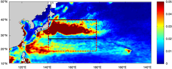
Fig. 1
Long-term mean (2006–2009) eddy kinetic energy (units: m2 s−2) in the North Pacific. The black rectangle area represents the KE region. The WRF model domain is represented by the red dashed rectangle area.
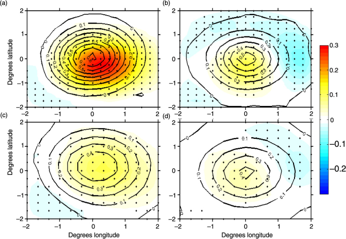
Fig. 2
Top panels: Composites of TMI SST anomalies (contours at the interval of 0.1 °C) and observational surface wind speed anomalies (shadings; units: m s−1). Bottom panels: CFSR reanalysis SST anomalies (contours at the interval of 0.1 °C) and CFSR surface wind speed anomalies (shadings; units: m s−1) for the warm eddies in winter (a, c) and summer (b, d). Areas with dots pass a two-tailed t test at the 0.05 level.
Table 1. Slopes of linear fits of some variables vs. SST anomalies
WinterSpringSummerAutumnWinterSpringSummerAutumn
Surface wind speed (ms−1 °C−1)0.3210.3240.2090.2230.3070.3190.2090.252CFSR surface wind speed (ms−1 °C−1)0.2230.2050.1320.1850.2200.2030.1190.179Sensible heat flux (W m−2 °C−1)15.25710.6385.8979.44915.69310.3965.8239.163CFSR sensible heat flux (W m−2 °C−1)16.66810.7945.6259.68716.73811.0825.5509.630Latent heat flux (W m−2 °C−1)23.14617.65613.59222.77722.37115.36113.76121.767CFSR latent heat flux (W m−2 °C−1)41.53429.68326.30040.88141.93829.82427.05741.059CFSR MABL height (m °C−1)47.73452.87856.13862.75650.78751.66866.97461.048
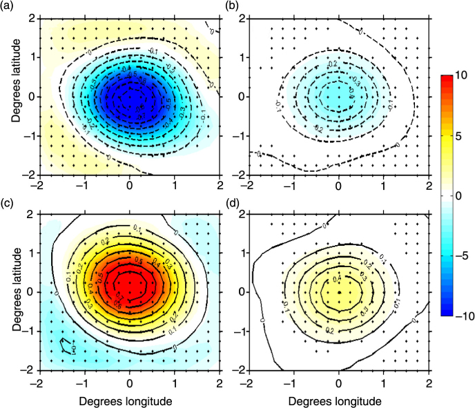
Fig. 3
Composites of TMI SST anomalies (contours at the interval of 0.1 °C) and J-OFURO sensible heat flux anomalies (shadings; units: Wm−2) for the cold (a, b) and warm (c, d) eddies in winter (a, c) and summer (b, d). Areas with dots pass a two-tailed t test at the 0.05 level.
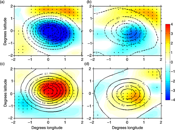
Fig. 4
Composites of TMI SST anomalies (contours at the interval of 0.1 °C) and cloud liquid water anomalies (shadings; units: 1×10⁻³ mm) for the cold (a, b) and warm (c, d) eddies in winter (a, c) and summer (b, d). Areas with dots pass a two-tailed t test at the 0.05 level.
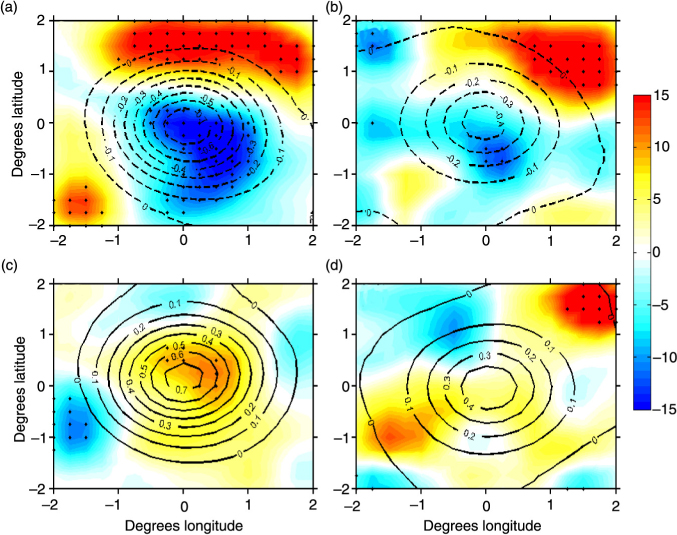
Fig. 5
Composites of TMI SST (contours at the interval of 0.1 °C) and rain rate anomalies (shadings; units: 1×10⁻³ mm h−1) for the cold (a, b) and warm (c, d) eddies in winter (a, c) and summer (b, d). Areas with dots pass a two-tailed t test at the 0.05 level.
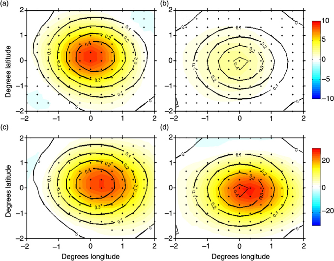
Fig. 6
Top panels: Composites of CFSR reanalysis SST anomalies (contours at the interval of 0.1 °C) and CFSR sensible heat flux anomalies (shadings; units: Wm−2). Bottom panels: Same contours as in the top panels and MABL height anomalies (shadings; units: m) for the warm eddies in winter (a, c) and summer (b, d). Areas with dots pass a two-tailed t test at the 0.05 level.
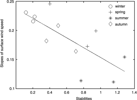
Fig. 7
Scatterplot of static stabilities and slopes of surface wind speed anomalies versus SST anomalies in the 12 calendar months.
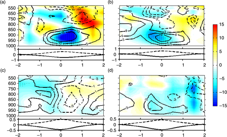
Fig. 8
Longitude-height cross-sections of the composite vertical transport anomalies of transient zonal momentum (units: 1×10⁻³ Pa m s−2) along the cold (shown in shadings) and warm (shown in contours) eddy centre's latitude in winter (a; contour interval of 5×10⁻³ Pa m s−2), spring (b; contour interval of 3×10⁻³ Pa m s−2), summer (c; contour interval of 2×10⁻³ Pa m s−2) and autumn (d; contour interval of 3×10⁻³ Pa m s−2). Areas with dots pass a two-tailed t test at the 0.05 level. Composites of SST anomalies along the cold (warm) eddy centre's latitude are shown in solid (dashed) lines below each cross-section.
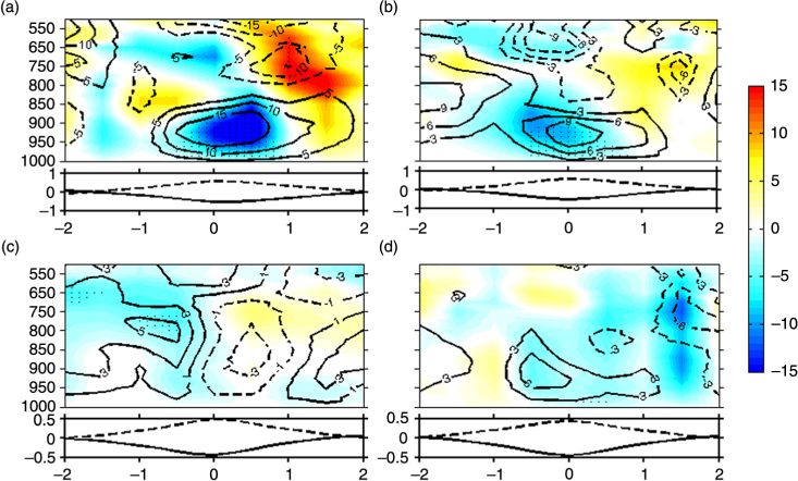
Fig. 9
Same as in Fig. 8, except for the composite wind speed anomalies (units: m s−1).
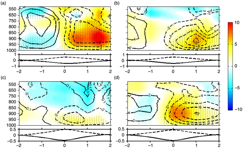
Fig. 10
Same as in Fig. 8, except for the composite vertical velocity anomalies (shadings; units: 1×10⁻³ Pa s−1).
Table 2. List of physics parameterisation schemes used in the WRF model
MicrophysicsWSM 3-class simple ice scheme (Dudhia et al., 2008)Longwave radiationRREM scheme (Mlawer et al., 1997)Shortwave radiationDudhia scheme (Dudhia, 1989)Surface layerMonin–Obukhov (Janjic Eta) scheme (Janjic, 2002)Land surfaceNoah scheme (Chen and Dudhia, 2001)Boundary layerMellor–Yamada–Janjic scheme (Janjic, 1994)Cumulus convectionKain–Fritsh scheme (Kain and Fritsch, 1993; Kain, 2004)
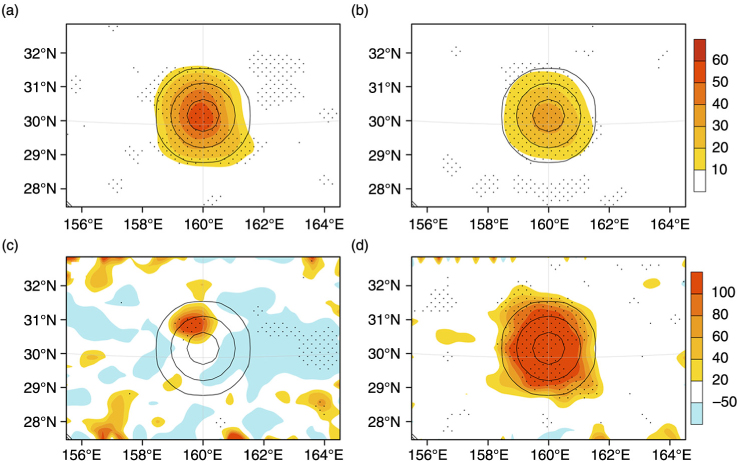
Fig. 11
SST differences (a–d; contours; units: °C), upward heat flux differences (a, b; shadings; units: W m−2) and MABL height differences (c, d; shadings; units: m) between the WE and CTL runs in winter (a, c) and summer (b, d). Areas with dots pass a two-tailed t test at the 0.05 level.
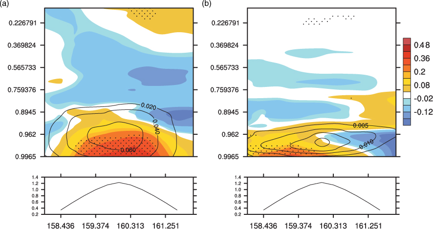
Fig. 12
Longitude-height cross-sections of wind speed differences (shadings; units: ms−1) and turbulent kinetic energy differences (contours; units: m2 s−2) between the WE and CTL runs along the eddy centre's latitude in winter (a; contour interval of 0.02 m2 s−2) and summer (b; contour interval of 0.005 m2 s−2). The vertical coordinate shows the model sigma levels. Areas with dots pass a two-tailed t test at the 0.05 level. Composite of SST differences along the eddy centre's latitude is shown below each cross-section.
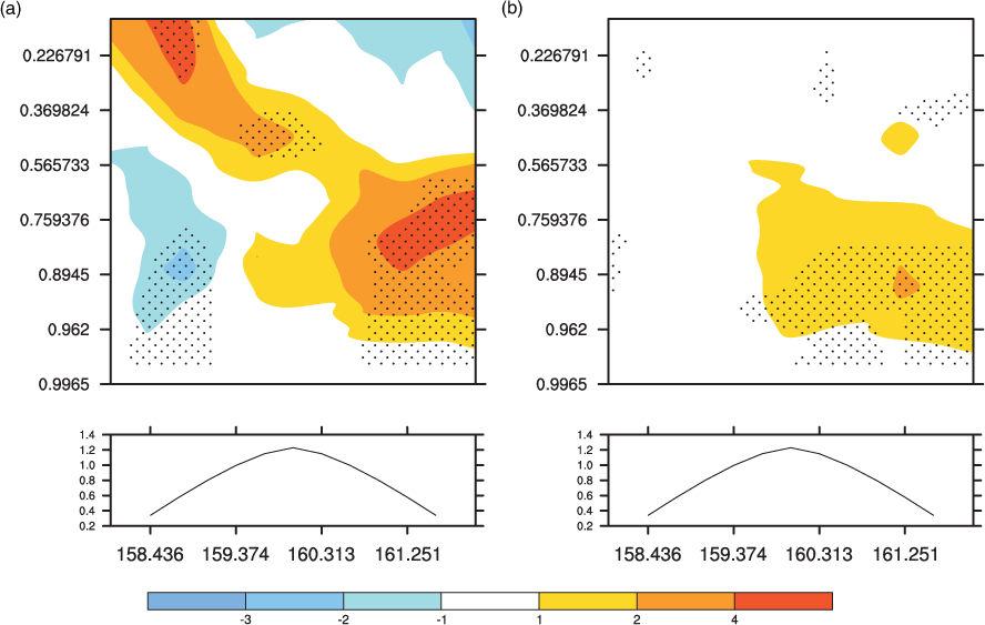
Fig. 13
Same as in Fig. 12, except for vertical velocity differences (shadings; units: 1×10⁻³ m s−1).
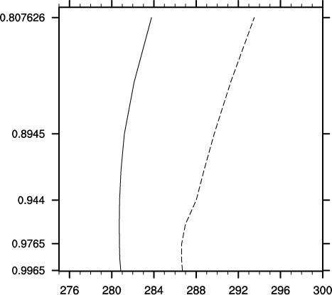
Fig. 14
Profiles of virtual potential temperature (units: K) averaged over the model domain in winter (solid line) and summer (dashed line) in CTL runs. The vertical coordinate refers to the model sigma levels.