
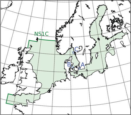
Fig. 1
FCOO NS1C model setup. Data comparison positions are marked for clarity: Drogden (A) at (longitude; latitude)=(12.7117; 55.5358), Ballen (B) at (10.6444; 55.8167) and Å13 (C) at (11.0333, 58.3367).
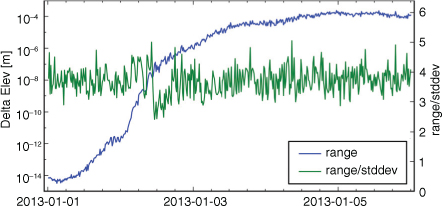
Fig. 2
Elevation RANGE (max − min results) at position ‘Ballen’, see Fig. 1 for position. Also shown is the ratio RANGE/STDDEV, where RANGE and STDDEV are computed over the 20 ensemble members.
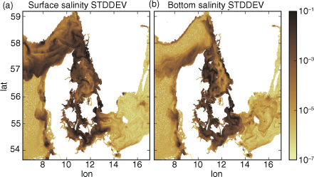
Fig. 3
Salinity variation (PSU) (STDDEV over 20 ensemble members) at surface (a) and bottom (b) after 5 d of simulation.
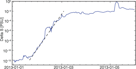
Fig. 4
Surface salinity RANGE (max − min over 20 ensemble members) time series at the Drogden Sill (the Sound).
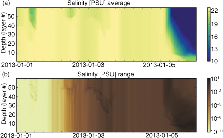
Fig. 5
Time-depth diagram of ensemble salinity AVG (a) and RANGE (b) at the Drogden Sill (the Sound). Water depth at the sill is approximately 8 m.
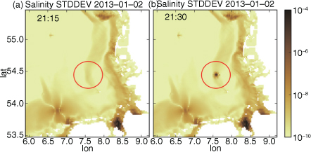
Fig. 6
Surface salinity variability (PSU) before (a) and after (b) a discrete ‘jump’ in a single ensemble member.
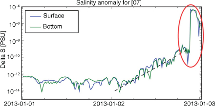
Fig. 7
Absolute value of the salinity anomaly of simulation #07 at (longitude, latitude)=(7.569, 54.441).
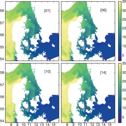
Fig. 8
Surface salinity (PSU) for 4 of 20 ensemble members after 2 months of simulation (2013-03-01).
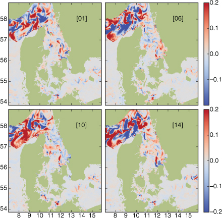
Fig. 9
Salinity anomaly (PSU) for 4 of the 20 members after 2 months of simulation (2013-03-01).
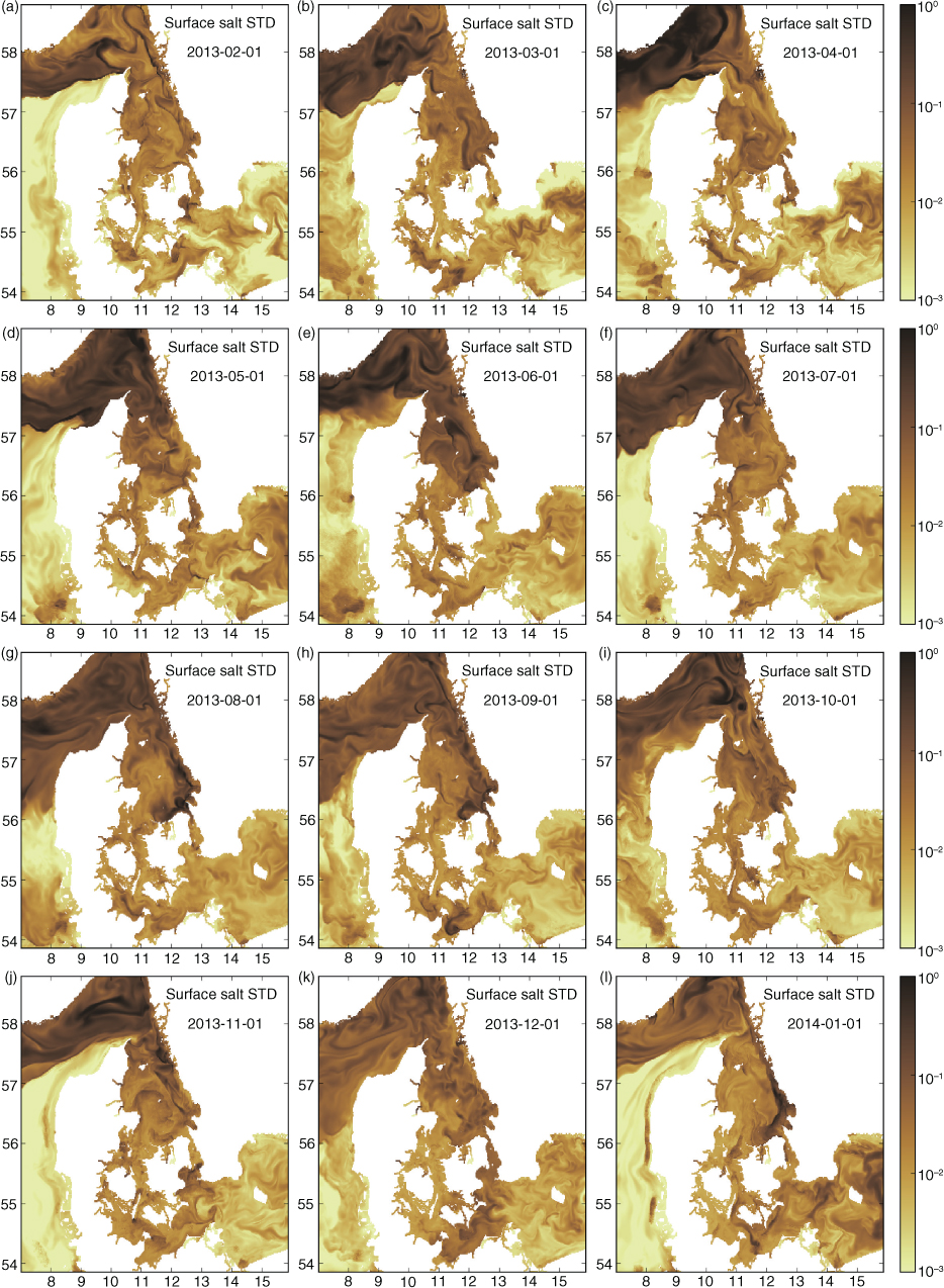
Fig. 10
Surface salinity STDDEV (PSU), σ SS, over 20 ensemble members at 1-month time interval.
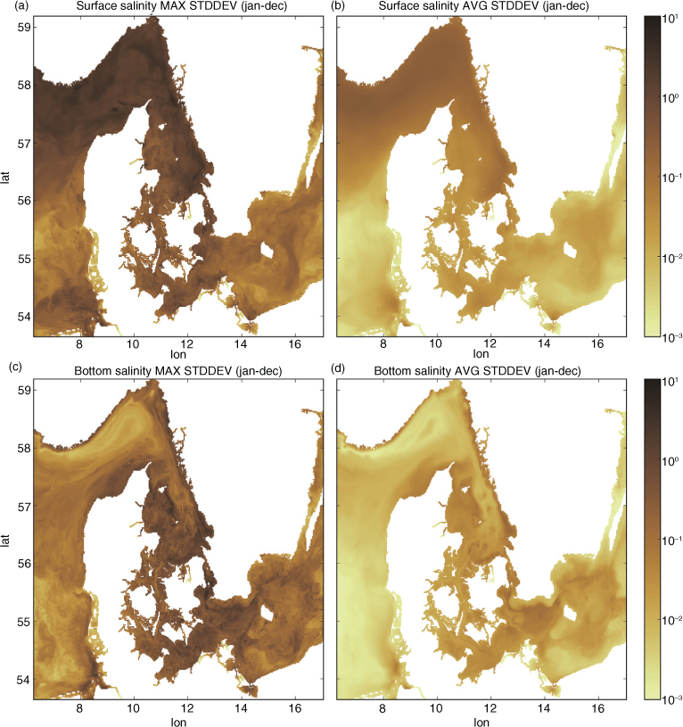
Fig. 11
Maximum surface salinity STDDEV (PSU) over time (a) and time-average (b) as well as time-maximum (c) and time-average (d) bottom salinity standard deviation over time for the 12-month simulation. Computations based on hourly values of salinity.
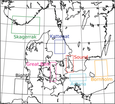
Fig. 12
Regions to compute time evolution of averaged and maximum standard deviation of salinity and temperature.
Table 1. Computed long-term ensemble variability for salinity and temperature for different areas
Depth (m)SurfaceBottomSurfaceBottom
Avg (area)Avg (area)Max (area)Avg (area)Max (area)Avg (area)Max (area)Avg (area)Max (area)
Skagerrak2901.4E-017.4E-017.2E-031.6E-017.9E-024.5E-013.1E-023.1E-01Kattegat285.7E-025.3E-013.8E-026.9E-012.2E-021.8E-014.9E-023.4E-01The Sound124.2E-024.4E-015.8E-028.9E-011.7E-022.4E-012.1E-021.8E-01Arkona391.9E-021.5E-014.7E-025.0E-012.1E-021.3E-013.6E-023.5E-01Great Belt172.2E-022.3E-012.2E-023.3E-016.8E-031.3E-017.6E-038.9E-02Bornholm721.8E-028.1E-022.3E-021.9E-013.7E-022.3E-014.9E-023.8E-01German Bight226.7E-038.5E-024.6E-037.0E-023.2E-033.8E-022.7E-032.3E-02
Table 2. Time scales (in days) to reach long-term ensemble variability (Table 1) for salinity and temperature for different areas
SurfaceBottomSurfaceBottom
Avg (area)Max (area)Avg (area)Max (area)Avg (area)Max (area)Avg (area)Max (area)
Skagerrak2118591819175548*Kattegat1847122*261711300*24The Sound284541510129*12Arkona4375*22545*24130137Great Belt5374667*4Bornholm543255187283*73*94*German Bight105*161010101311
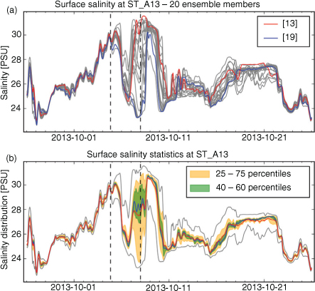
Fig. 13
Time series of surface salinity at position ‘Å13’ in eastern Skagerrak from September 26 to October 26. Surface salinity of the 20 ensemble members, highlighting two particular members (a), and time series of statistical properties (b) including minimum and maximum values (grey), median (blue) and mean (red) values, and two percentile intervals. Dashed black lines indicate times used in later figures: 2013-10-04 20:00 and 2013-10-08 00:00.
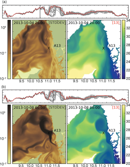
Fig. 14
Surface salinity in eastern Skagerrak on 2013-10-04 20:00 (a) and 2013-10-08 00:00 (b), where X indicates the location for position ‘Å13’. Sea surface salinity STDDEV (PSU) (left) and surface salinity (PSU) for ensemble member #13 (right). In each subfigure, the top panel indicates time in a way consistent with Fig. 13.
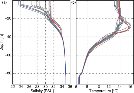
Fig. 15
Vertical profiles of salinity (a) and temperature (b) for individual ensemble members on 2013-10-08 at position ‘Å13’. Members #13 (red) and #19 (blue) are highlighted identical to Fig. 13a.
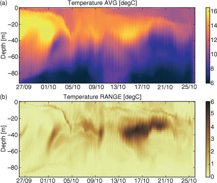
Fig. 16
Time-depth plot of salinity AVERAGE (a) and RANGE (b) over the ensemble at position ‘Å13’.
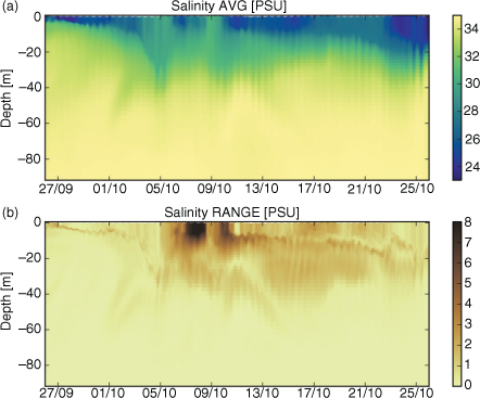
Fig. 17
Time-depth plot of temperature AVERAGE (a) and RANGE (b) over the ensemble at position ‘Å13’.