
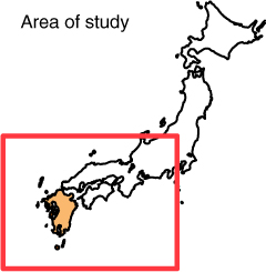
Fig. 1
Area of study in south-west Japan (red solid box) used to define the atmospheric patterns. The orange shading represents the Kyushu region used in Section 3b.
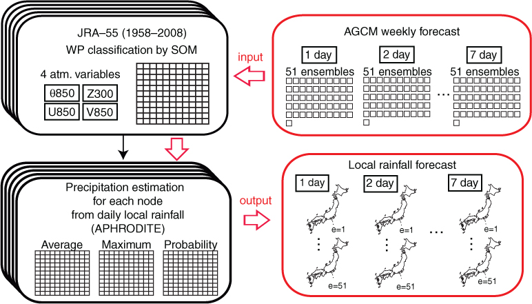
Fig. 2
Schematic diagram of the SOM-based downscaling method. The five different SOM classifications of the WP are based on the normalised anomalies of four atmospheric variables for June–July and August–September during 1958–2009 (top left). Based on the SOM lattices, the precipitation PDF patterns are estimated for each node (bottom left). By using the SOM lattice, the downscaled precipitation is obtained (bottom right) from the 51 daily members of the EPS produced for 7 d (top right).
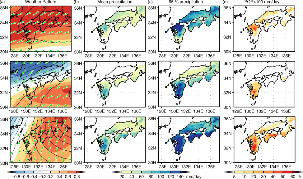
Fig. 3
Three examples of anomalous WPs derived from the 20×20 SOM non-linear classification. (a) Node-averaged (composited) daily-mean 850-hPa θe (K: red–blue shading), 300-hPa GH (m: black contour) and 850-hPa wind (m/s: green vectors) anomalies. The WP-related (b) mean precipitation, (c) 95th percentile precipitation and (d) 100 mm/day rainfall rate (%; probability of precipitation) for each node.
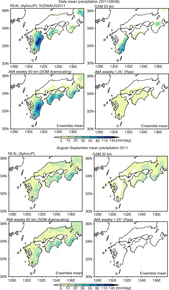
Fig. 4
(a) Daily mean precipitation (mm/day) on 6 August 2011 for observed, 20 km GSM (no ensemble), SOM downscaling (ensemble mean) and 60-km GSM (ensemble mean). (b) is same as (a) except for August–September.
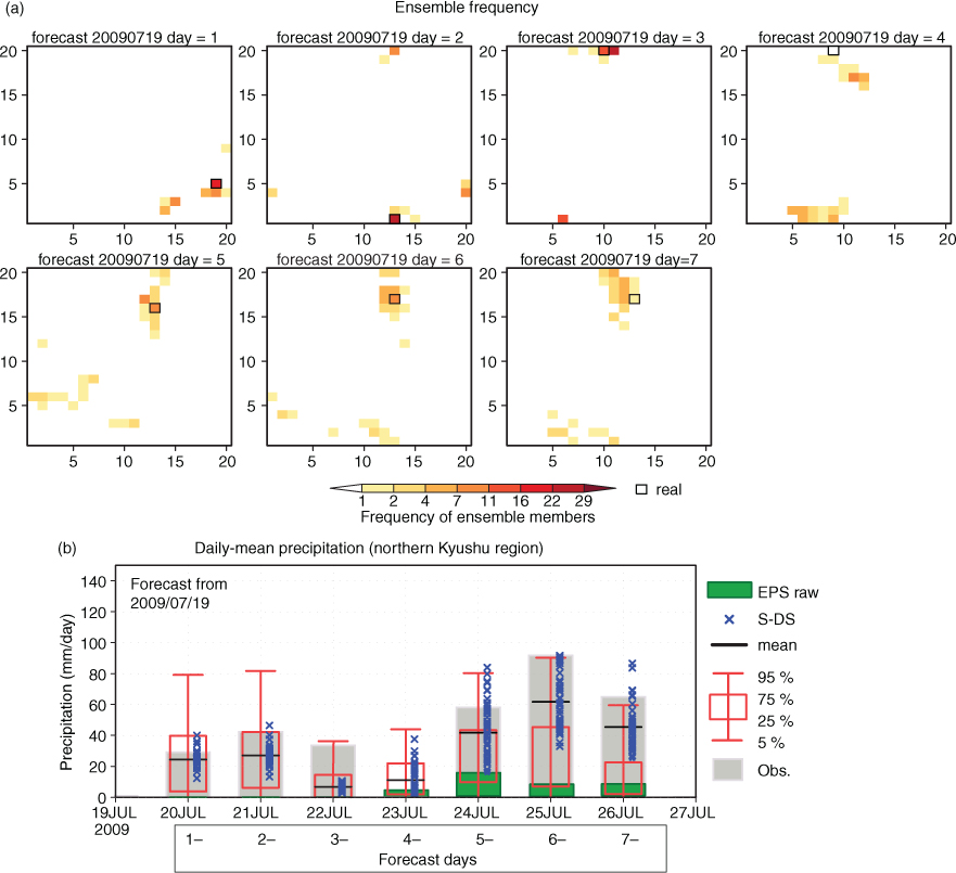
Fig. 5
(a) SOM frequency (best matched) of the 51 ensemble members on the 20×20 SOM lattice for forecast days 1–7. Solid black box represents the actual state. (b) Daily mean precipitation obtained from the downscaling for forecast days 1–7. The spread of the ensemble for GSM raw is presented by the green-shaded box (EPS raw). The node-mean downscaled precipitation (S-DS) and its ensemble mean are represented by black ‘×’ mark and horizontal bar, respectively. Composited PDFs of downscaled precipitation obtained from the SOM are represented by red error bar. Observational precipitation (actual state) is represented by the grey bar.
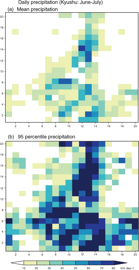
Fig. 6
Daily precipitation (mm/day) averaged over the Kyushu region for (a) node-mean and (b) 95th percentile on the 20×20 SOM lattice during June–July.
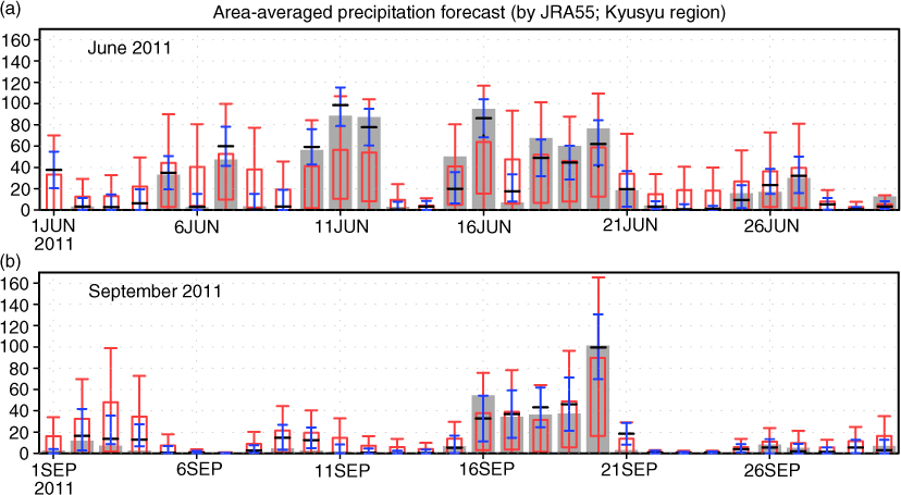
Fig. 7
Forecasted daily mean precipitation obtained from the downscaling by using JRA-55 as predictor during (a) June and (b) September 2011. Black horizontal bar represents the estimated precipitation by the substatistical model and the error bar 2-sigma. Composited PDFs of downscaled precipitation obtained from the best-match SOM nodes are represented by red error bar (5th, 25th, 75th and 95th percentiles). Observational precipitation (actual state) is represented by the grey bar.
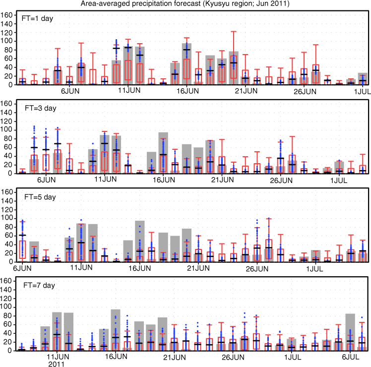
Fig. 8
Same as Fig. 7 except for forecast day 1, 3, 5 and 7 of EPS during June 2011. The downscaled precipitation by the substatistical model and its ensemble mean are represented by blue dots and black horizontal bars, respectively.
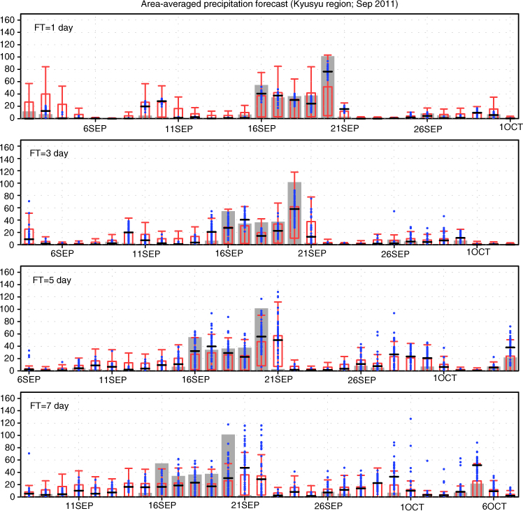
Fig. 9
Same as Fig. 8 except for September 2011.
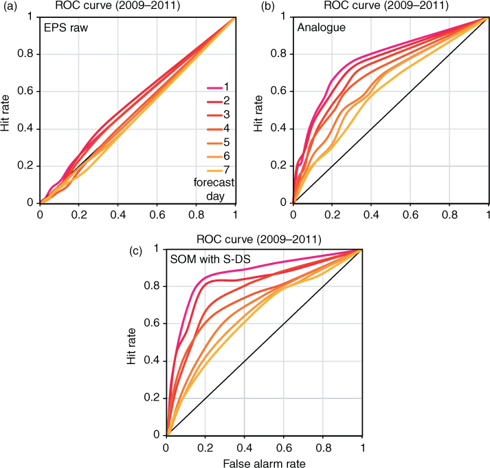
Fig. 10
ROC curves for forecast days 1–7 for the precipitation of (a) GSM raw, (b) analogue method and (c) SOM downscaling for the periods of June–July and August–September in 2009–2011.
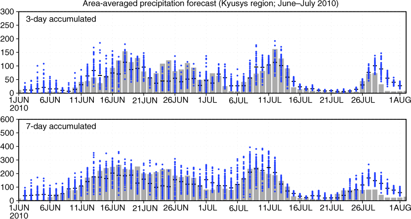
Fig. 11
Same as Fig. 8 except for forecast 3-d and 7-d accumulated precipitation in June–July 2010.
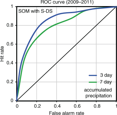
Fig. 12
ROC curves for the forecast 3-d and 7-d accumulated precipitation of SOM downscaling for the periods June–July and August–September in 2009–2011.