
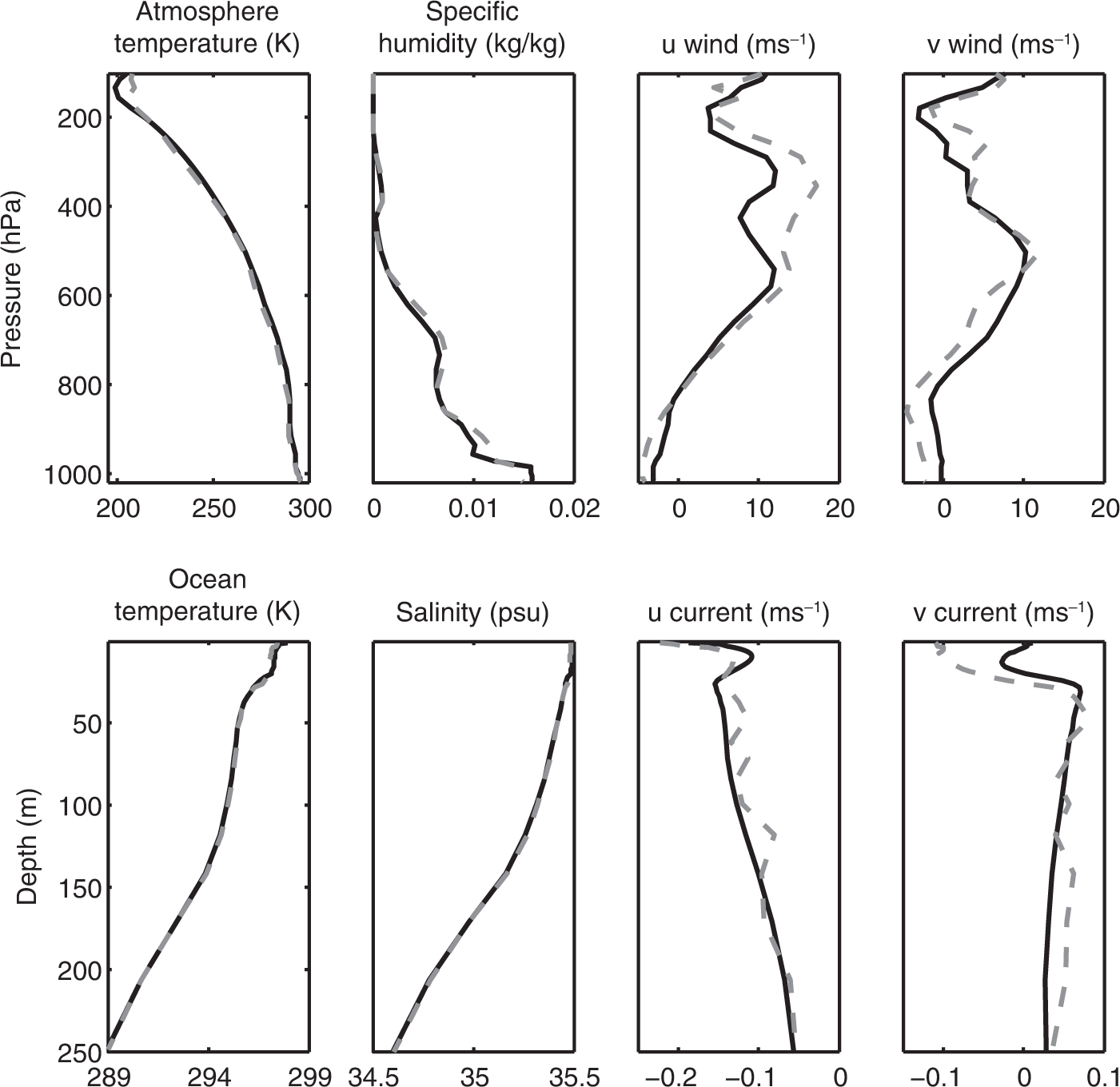
Fig. 1
True (solid black line) and background (dashed grey line) initial states.
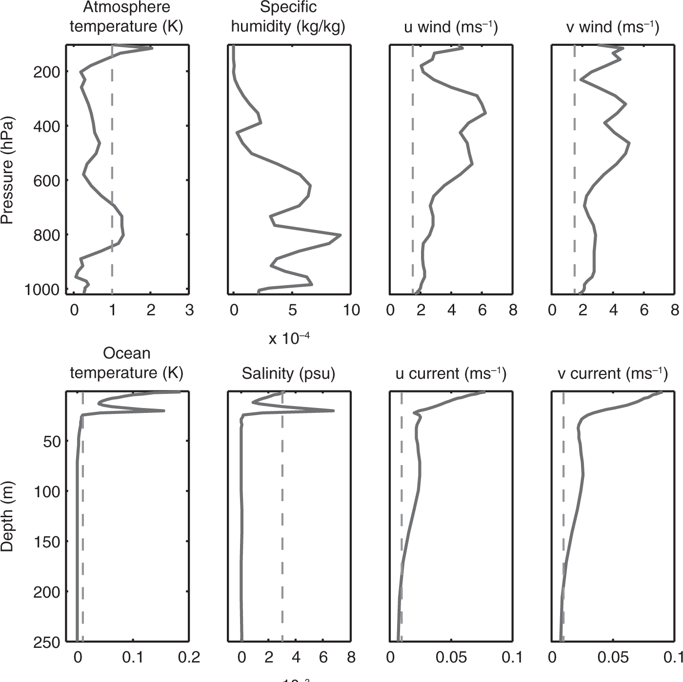
Fig. 2
Initial background (solid grey line) and observation (vertical dashed grey line) error standard deviations.
Table 1. Observation error standard deviations by field
1.01.51.50.010.0030.010.01
Table 2. Atmosphere observation locations
14109.893172018.815193028.882225054.624237066.6232510095.98028150154.03830200202.23032250257.68533300288.09336400389.23339500501.63744700694.69649850861.49752925935.065561000995.05560n/a1017.293
Table 3. Ocean observation locations
11.00033.06955.27788.8481011.4061315.5381620.1731823.7622028.1002233.7602337.3662441.7032546.9852653.4752761.4982871.4522983.8183099.17531118.21432141.75833170.77834206.41435250.000
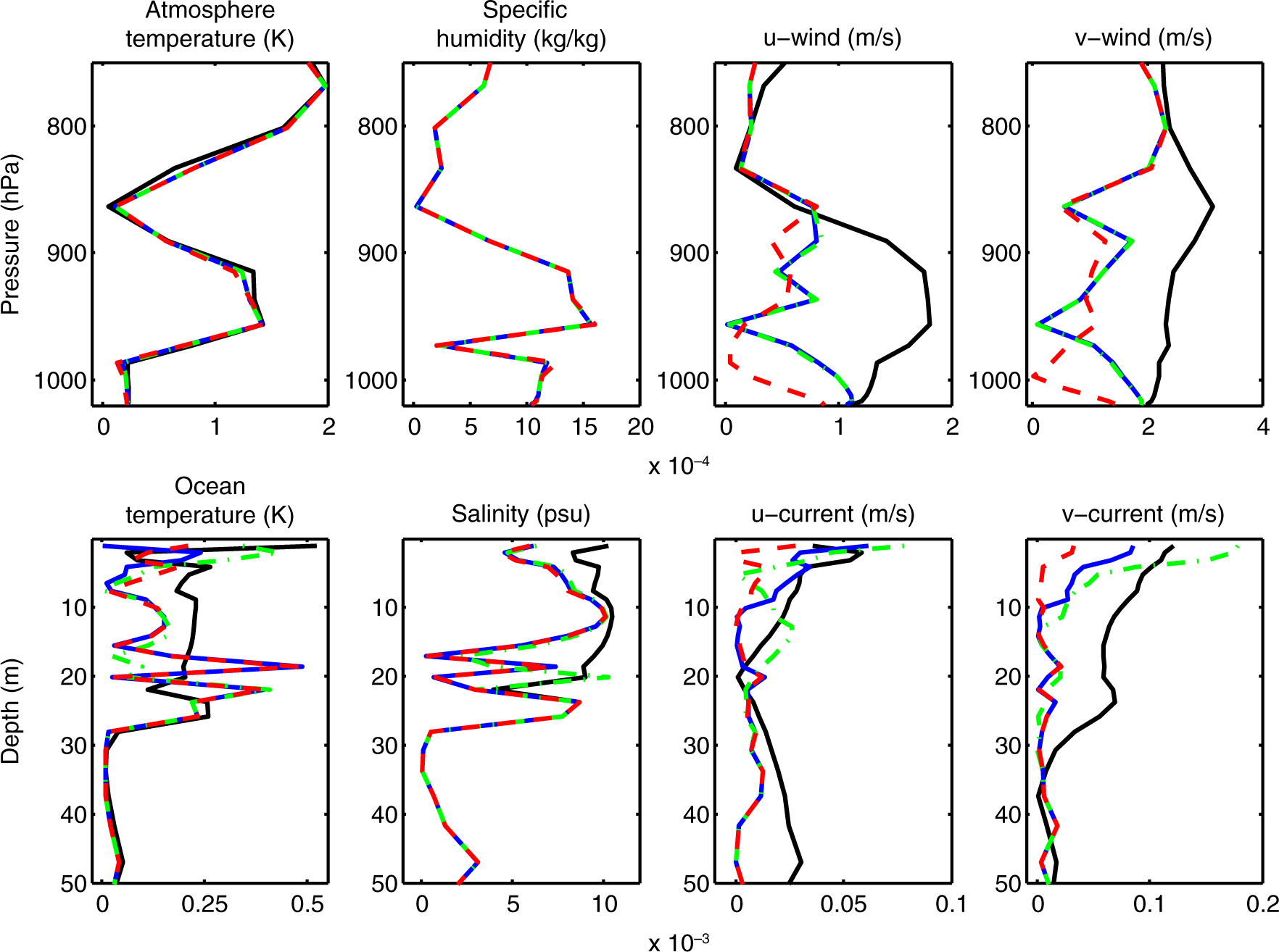
Fig. 3
Absolute errors at initial time: background error (solid black line), strongly coupled analysis error (dashed red line), weakly coupled analysis error (solid blue line), and uncoupled analysis error (dot–dash green line). Experiments using a 12-hour assimilation window with 3-hourly atmosphere & 6-hourly ocean observations. Observation locations are given in Tables 2 and 3.
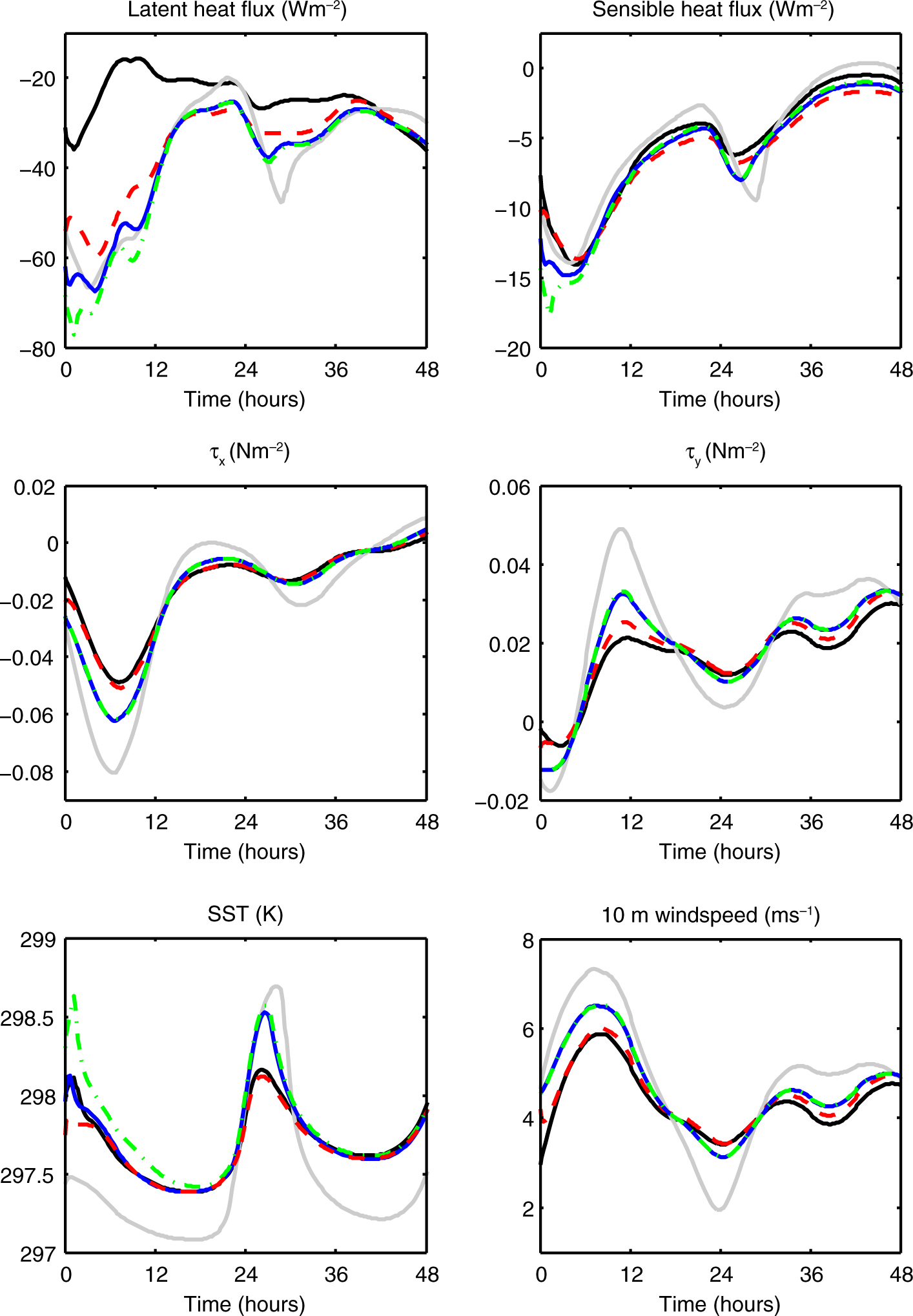
Fig. 4
Coupled model SST & surface fluxes for coupled model forecast initialised from t 0 analyses, first 48 hours of forecast: truth (solid black line), forecast initialised from initial background state (solid grey line), forecast initialised from strongly coupled analysis (dashed red line), forecast initialised from weakly coupled analysis (solid blue line), and forecast initialised from uncoupled analyses (dot–dash green line). Experiments using a 12-hour assimilation window with 3-hourly atmosphere & 6-hourly ocean observations.
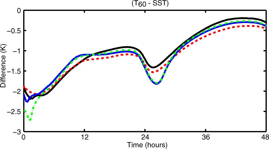
Fig. 5
Atmosphere–Ocean temperature difference (T 60–SST) for coupled model forecast initialised from t 0 analyses: truth (solid black line), forecast initialised from strongly coupled analysis (dashed red line), forecast initialised from weakly coupled analysis (solid blue line), and forecast initialised from uncoupled analyses (dot–dash green line). Experiments using a 12-hour assimilation window with 3-hourly atmosphere & 6-hourly ocean observations.
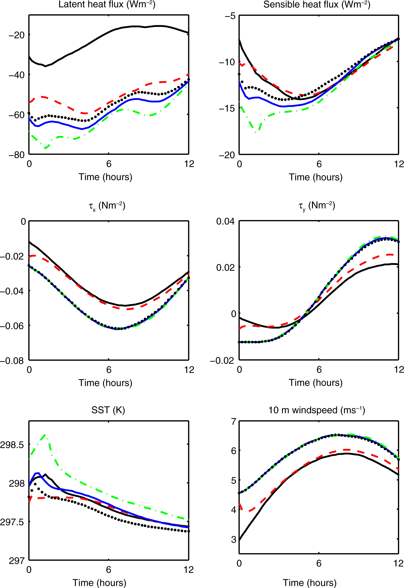
Fig. 6
Coupled model SST & surface fluxes for coupled model forecast initialised from t 0 analyses, first 12 hours of forecast: truth (solid black line), forecast initialised from strongly coupled analysis (dashed red line), forecast initialised from weakly coupled analysis (solid blue line), forecast initialised from uncoupled analyses (dot–dash green line), and forecast initialised from uncoupled analyses using ‘true’ forcing (black dots). Experiments using a 12-hour assimilation window with 3-hourly atmosphere & 6-hourly ocean observations.

Fig. 7
Coupled model SST & surface fluxes for coupled model forecast initialised from t 0 analyses, first 48 hours of forecast: truth (solid black line), forecast initialised from initial background state (solid grey line), forecast initialised from strongly coupled analysis (dashed red line), forecast initialised from weakly coupled analysis (solid blue line), and forecast initialised from uncoupled analyses (dot–dash green line). Experiments using a 12-hour assimilation window with 6-hourly atmosphere & 6-hourly ocean observations.

Fig. 8
Coupled model SST & surface fluxes for coupled model forecast initialised from t 0 analyses, first 12 hours of forecast: truth (solid black line), forecast initialised from initial background state (solid grey line), forecast initialised from strongly coupled analysis (dashed red line), forecast initialised from weakly coupled analysis (solid blue line), and forecast initialised from uncoupled analyses (dot–dash green line). Experiments using a 12-hour assimilation window with 6-hourly atmosphere & 6-hourly ocean observations.
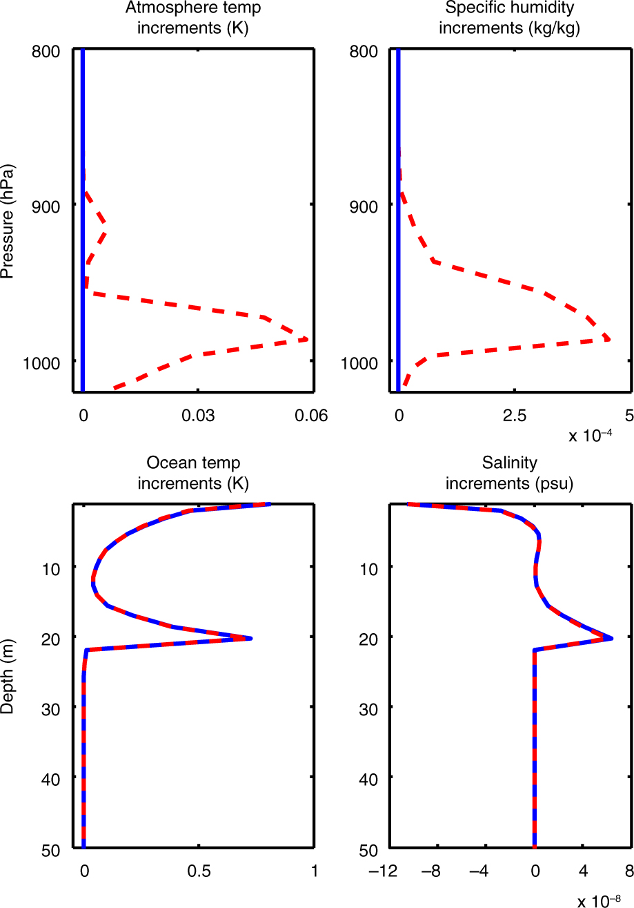
Fig. 9
Analysis increments at t=0: strongly coupled (dashed red line) and weakly coupled (solid blue line) assimilations with single SST observation at the end of a 12-hour assimilation window.
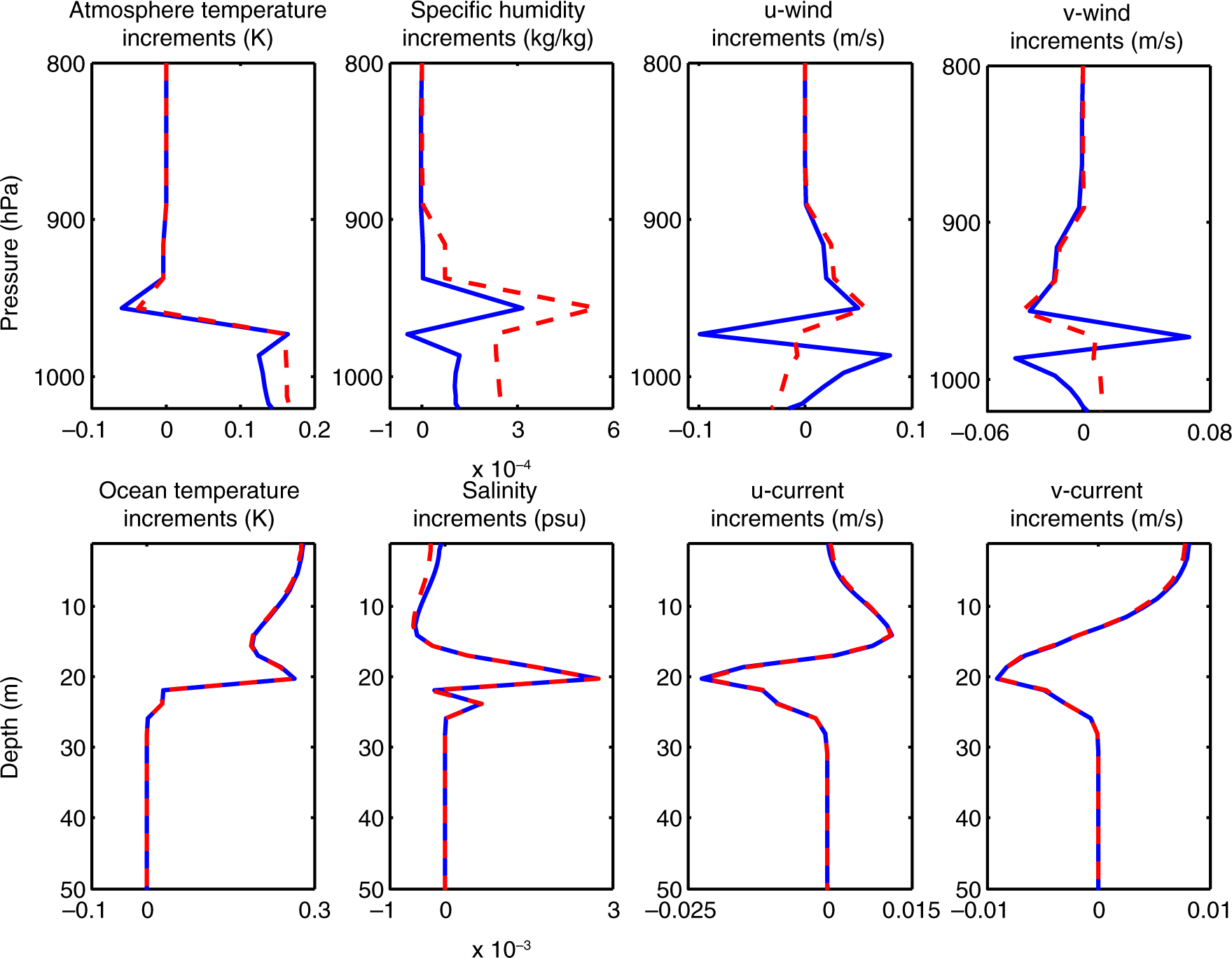
Fig. 10
Analysis increments at t=6 hours: strongly coupled (dashed red line) and weakly coupled (solid blue line) assimilations with single SST observation at the end of a 12-hour assimilation window.
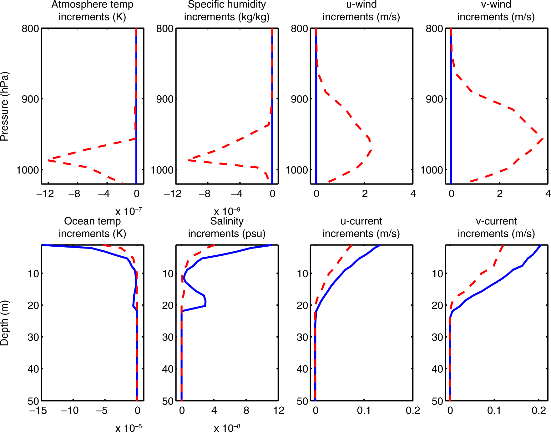
Fig. 11
Analysis increments at t=0: strongly coupled (dashed red line) and weakly coupled (solid blue line) assimilations with single ocean surface current observation at end of 12-hour assimilation window.
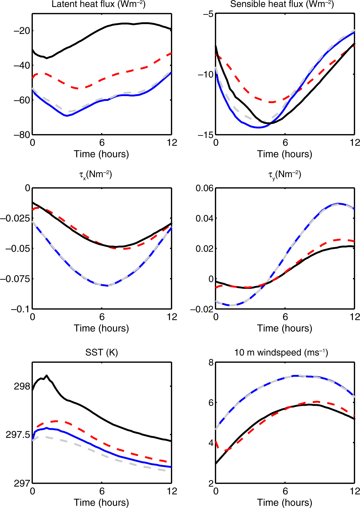
Fig. 12
SST & surface fluxes: truth (solid black line), initial background trajectory (dashed grey line), strongly coupled analysis (dashed red line) and weakly coupled analysis (solid blue line) from experiment with single ocean surface current observation at the end of a 12-hour assimilation window.
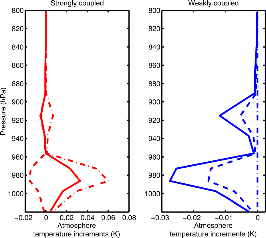
Fig. 13
Atmospheric temperature analysis increments at t=0: strongly coupled (left) and weakly coupled (right) assimilations with two observations of temperature, corresponding to the lowest model level in the atmosphere and the top model level in the ocean, at the end of a 12-hour assimilation window. The solid lines indicate the analysis increment when both temperature observations are assimilated; the dashed lines correspond to assimilation of the atmosphere temperature observation only; and dot–dash lines correspond to assimilation of the ocean temperature observation only.