
1. Introduction
The incoming solar irradiance, which is absorbed by the upper ocean, is the main energy source in the ocean heat budget, and hence strongly impacts the oceanic thermal structure, heat transport and the global circulations. Shortwave radiation is attenuated exponentially with depth. The attenuation depth (e-folding depth) depends on the wavelength and biogenic components of the water. Traditionally, the water types are classified Jerlov I, IA, IB, II and III (Jerlov, 1976). The shortwave attenuation depth (SWAD) in open oceans (almost Jerlov I) is about 20–30 m, and it decreases with increasing water turbidity, particularly in coastal regions.
So far a variety of solar transmission parameterisations have been developed for modelling ocean radiant heating (e.g. Simpson and Dickey, 1981; Morel and Antonine, 1994; Ohlmann and Siegel, 2000; Ohlmann, 2003; Kara et al., 2005). These parameterisations use the classic or hybrid Jerlov water type, chlorophyll concentration or photosynthetically active radiation (PAR), to estimate the SWAD. PAR is sunlight which is available for photosynthesis by phytoplankton (Liu et al., 1994). In general, most shortwave penetration schemes account for at least two shortwave bands: ‘red’ (wavelength more than 750 nm) and ‘blue’ bands (wavelength 300–750 nm) (e.g. Morel and Antonine, 1994; Ohlmann, 2003; Kara et al., 2005; Manizza et al., 2005; Ishizaki and Yamanka, 2010). Almost 98% of red and near-infrared radiation is absorbed within 2 m of the sea surface, but the visible and ultraviolet bands can penetrate much deeper (Kara et al., 2005). The attenuation of red or near-infrared wavelengths cannot be resolved into distinct layers if an ocean general circulation model (OGCM) has a fairly coarse vertical resolution. For example, the first layer in most OGCMs is greater than 2 m at present due to the limitations of current computer resources and numerical methods. So a simple approach, which considers penetration by the blue band only and uses a single exponential profile in the water column, is commonly used in OGCMs with typical vertical resolution (Murtugudde et al., 2002).
The solar penetrative radiation plays an important role in the upper-ocean dynamics and thermodynamics. There exists extensive literature exploring how the different light e-folding depth or shortwave penetration schemes impact the climate mean state and interannual variability in climate models, for ocean models alone and for coupled models. Murtugudde et al. (2002) investigated the differences of model performance between a constant attenuation depth (control run) and annual mean spatially varied depths derived from remotely sensed ocean colour data in an ocean model. The model with spatially varied depth, which is more realistic than a constant depth, can significantly reduce the sea surface temperature (SST) errors which are differences between model results and the corresponding observations compared to the control run. Ballabrera-Poy et al. (2007) extended the Murtugudde et al. (2002) study in a hybrid coupled atmosphere–ocean model. Two experiments were the same as those in Murtugudde's work, but the spatially varied SWAD in the third experiment included a seasonal cycle. It was found that the seasonal cycle of the SWAD interacted with the low-frequency equatorial dynamics to enhance warm and cold anomalies, which were further amplified via positive air–sea feedbacks. However, the model annual mean state was hardly affected by the different SWADs, since the atmospheric model is statistical and only provides the wind stress anomaly.
A few studies have undertaken sensitivity experiments with different SWADs using fully coupled climate models. Wetzel et al. (2006) investigated the influence of phytoplankton on the seasonal cycle and the mean global climate. Their control run used a fixed 11 m attenuation depth while the SWAD in the other experiment was derived from phytoplankton concentrations generated by a marine biogeochemical model coupled online to the ocean model, which has both seasonal cycle and interannual variability. Compared to the control run, they found that the experiment accounting for the impact of the marine biology on the radiative budget of the upper ocean could amplify the seasonal cycle, warm SSTs in the upwelling region, and improve El Niño and La Niña simulation in period and phase locking. Anderson et al. (2007) suggested a potential positive feedback between chlorophyll concentration and a non-local-coupled response based on a suite of surface chlorophyll perturbation experiments. Gnanadesikan and Anderson (2009) investigated the impact of ocean water clarity on the ocean general circulation in a fully coupled climate model.
Some studies have explored the role of different shortwave penetration schemes on model climate and oceanic circulations (e.g. Sweeney et al., 2005; Yamanaka et al., 2012). Sweeney et al. (2005) explored the effect of two different schemes on climate model simulations with an OGCM. One was the Ohlmann (2003) scheme and the other the Morel and Antonie (1994), hereafter MA. The Ohlmann scheme estimated a deeper SWAD than the MA scheme did. The model with the Ohlmann scheme (greater SWAD) produced a slowdown in the heat transport (5%) between the tropics and subtropical upper oceans compared to the model with the MA scheme. Sweeney et al. (2005) suggested that this slowdown was primarily due to off-equatorial increases in the mixed layer depth (MLD).
Here we will perform experiments using an OGCM with different estimates of SWAD derived from remotely sensed ocean colour data. The differences of SWAD are caused by different algorithms for converting attenuation depth at 490 nm to SWAD. Previous work of Murtugudde et al. (2002), Ballabrera-Poy et al. (2007) and Wetzel et al. (2006) compared the model climates between a constant attenuation depth and a spatially varied SWAD. All of the SWADs used in this study are spatially varied and include a seasonal cycle. Sweeney et al. (2005) applied seasonal-variation chlorophyll dataset from Sea-viewing Wide Field-of-view Sensor (SeaWiFS) for two shortwave penetration schemes which estimate different SWADs. They integrated the ocean model for only 10 years forced with a climatological forcing and the model interannual variations were ignored. Our ocean model will be forced with an interannual forcing for almost 60 years. The objective of this paper is to explore how the different SWADs impact the model's climate mean state and interannual variations, and investigate the causes for the differences in temperature and ocean currents due to the different SWADs.
This paper is organised as follows. Section 2 describes the satellite data and the two algorithms used to estimate the SWAD. The OGCM used here and experiment design are described briefly in Section 3. The model results based on different estimates of SWAD are presented in Section 4 and, finally, Section 5 provides a summary and some discussions.
2. Estimates of shortwave penetration depths from SeaWiFS
The SeaWiFS project has provided quantitative data on global ocean bio-optical properties to the Earth science community (Cracknell et al., 2001). SeaWiFS began scientific operations in September 1997 and stopped collecting data in December 2010. The diffuse attenuation coefficient at 490 nm [K d(490)] can be estimated from the SeaWiFS dataset using the algorithm described in Werdell and Bailey (2005). There is strong pigment absorption at 490 nm by phytoplankton and the solar irradiance at this wavelength controls the rate of photosynthesis. The downward diffuse attenuation coefficient (inverse of SWAD) for the K d (PAR) can be estimated with different algorithms based on the retrieved K d(490) data from the SeaWiFS data (Morel et al., 2007; Pierson et al., 2008; Wang et al., 2009; Saulquin et al., 2013). The K d (PAR) estimates proposed by Morel et al. (2007) with two different algorithms are suitable for clear water in open oceans, whereas the calculations of K d (PAR) suggested by Pierson et al. (2008) and Wang et al. (2009) are only valid for special coastal regions such as Cheasapeake Bay turbid waters and Baltic Sea. The scheme for K d (PAR) proposed by Saulquin et al. (2013) is, in fact, close to one of two algorithms from Morel et al. (2007). Therefore, we apply the estimates of K d (PAR) in Morel et al. (2007) to investigate how an ocean climate model responds the different SWADs. The K d (PAR) depends significantly on the thickness of the layer considered, since, due to varying attenuation rate with wavelength, the PAR domain narrows down deeper in the water column and, finally, concentrate around the least attenuated wavelength. The regression equation relating K d (PAR) to K d(490) depends on the different thicknesses of the top layer which can be defined as or its double. If the top layer is equal to the first penetration depth of thickness , the best fit for K d (PAR) is
If the top layer considered is increased to double penetration depth of , K d (PAR) will decrease as belowThese are the two formulations derived by Morel et al. (2007). The inverse of K d (PAR), is the SWAD.Figure 1 shows the relationship between the and from eqs. (1) and (2). The depth of is close to double that of in most cases, since the PAR is the polychromatic radiation within the entire 400–700 nm spectral range (Tyler, 1966). The diffuse attenuations depend on the wave length and chlorophyll concentration. Within the PAR spectral range, the blue light at 490 nm has the smallest diffuse attenuation coefficient and penetrates furthest in the clear water. Where chlorophyll concentrations are high, such as in coastal regions, , and converge at around 5 m. However, is smaller than , and their difference will become larger in open oceans with oligotrophic waters. The solid line in Fig. 1 shows the average of and .
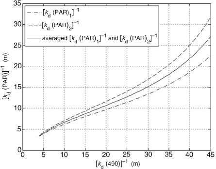
Fig. 1
The relationship of attenuation depth (m) at 490 nm and different estimates of depth of photosynthetically active radiation (PAR).
Figure 2 displays the spatial distribution of the annual mean , , and the difference between and from the SeaWiFS dataset. Their patterns look similar to each other. Low values are found in the coastal regions and the upwelling zones in the eastern equatorial pacific and Atlantic oceans. High values are found in the subtropical gyres where biological productivity is low. is almost two times deeper than in most oceans. is generally around 6–10 m deeper than in the subtropical area and 2–4 m deeper along the equatorial regions. Note that the estimation of SWAD proposed by Saulquin et al. (2013) [eqs. (9a) and (9b)] is deeper than here almost everywhere in the open ocean, for example, about 5 m deeper during the range from 25 to 35 m for .
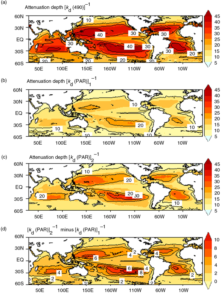
Fig. 2
Attenuation depths (m) for 490 nm (a), (b) and (c) estimated from SeaWiFS during the period of 1997–2010 and (d) is the differences between and .
3. The climate model and experimental design
3.1. Model description
The ocean component of the Australian Community Climate and Earth System Simulator (ACCESS-OM; Bi et al., 2013) is used here for model experiments. ACCESS-OM comprises the United States (US) National Oceanographic and Atmospheric Administration (NOAA) Geophysical Fluid Dynamics Laboratory (GFDL) Modular Ocean Model version 4.1 (MOM4p1; Griffies, 2009), the US Los Alamos National Laboratory version 4.1 sea-ice model CICE (Community Ice CodE, Hunke and Lipscomb, 2010) and the OASIS3.25 coupler (Valcke, 2006).
The horizontal resolution of the ocean model is a uniform 1° in the longitudinal direction. In the meridional direction, the grid spacing is nominally 1° resolution with three refinements: (1) 1/3° between 10°S and 10°N; (2) tripolar Arctic north of 65°N; and (3) a Mercator (cosine-dependent) implementation for the southern hemisphere ranging from 0.25° at 78°S to 1° at 30°S. The vertical discretisation has 50 levels covering 0–6000 m. In the top 200 m, the resolution is uniform with a grid spacing of 10 m. Below 200 m, vertical grid spacing increases linearly to 330 m at the bottom-most tracer cell. The vertical mixing scheme is a non-local K-profile parameterisation (Large et al., 1994). Lateral friction is parameterized using a combination of biharmonic and Laplacian viscosity (Griffies and Hallberg, 2000).
3.2. Shortwave penetration scheme
The solar subsurface heating parameterisation used here was proposed by Kara et al. (2005). Its formula is represented as
where γ=max(0.27,0.695−5.7*K d(PAR)), Q(0) is the net heat flux absorbed at the sea surface, Q(z) is remaining heat flux at depth z, γ is the fraction of solar radiation in the blue band and K d(PAR) is the shortwave diffuse coefficient as appropriate for eqs. 1 and 2.3.3. Experimental design
The atmospheric forcing used here is an updated version 2 Coordinated Ocean-ice Reference Experiments (COREv2) interannual forcing dataset (Large and Yeager, 2009). The COREv2 dataset provides the air temperature, winds, air specific humidity, rainfall rate and snowfall rate, pressure at 10 m, downward shortwave radiation, downward longwave radiation and river runoff. These data have a global coverage and start from 1948 at frequencies ranging from 6-hourly to monthly. All fluxes are computed over the 23 yr from 1984 to 2006, but radiation prior to 1984 and precipitation before 1979 are given only as climatological mean annual cycles.
Three experiments, which are denoted EX1, EX2 and EX3, are conducted using ACCESS-OM. They employK d(PAR)1, K d(PAR)2 and K d(AVE), respectively. K d(AVE) is a reciprocal of the average attenuation depth of and . All experiments are forced with COREv2 atmospheric forcing during the period of 1948–2007. They are initialised with observed climatological temperatures and salinities from the NOAA World Ocean Atlas 2005 (WOA05; Antonov et al., 2006; Locarnini et al., 2006). No SST restoring scheme is applied here, but a 60 d linear sea surface salinity (SSS) restoring over the upper model layer is used to reduce model salinity drift.
4. Results
We investigate how the different SWADs impact on the model simulations in temperature fields, sea surface height (SSH), MLD, 20°C isotherm depth (D20) and circulation. The model is spun up from 1948, but the results during the period of 1980–2007 are used for analysis in this study.
4.1. Analysis of temperature
4.1.1. Model temperature errors.
The vertical profiles of temperature errors for all experiments are illustrated in Fig. 3. They are averaged horizontally within the domain of 30°S to 30°N, since the SWAD differences for all experiments are large in this region (Fig. 2d). The three runs have similar and small cold biases near the sea surface, since the sea surface simulations are largely controlled by the external atmospheric forcing such as wind stress, heat flux etc. At 50 m, experiment EX1 has the largest cold bias (up to 0.4°C) while experiment EX2 has a small error at this depth. At depths of 150 to 200 m, EX2 has a large warm bias (about 0.5°C), while EX1 has a small error here. The temperatures in EX2 are warmer than those in EX1 over the upper 500 m except near the sea surface; the greatest differences occur at depths ranging from 50 to 200 m. The value of the SWAD in EX3 is the average of the SWADs of EX1 and EX2. It is interesting, therefore, that the vertical temperature errors in EX3 are almost near the midpoint between the errors of EX1 and EX2. This indicates that, to a large extent, the model temperature simulation has a linear response to the different SWADs in the upper oceans.
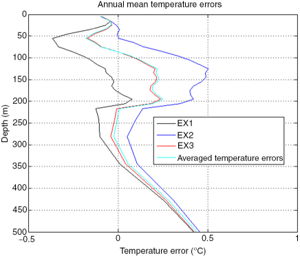
Fig. 3
The mean temperature errors (°C) averaged zonally within 30°S–30°N for EX1 (blue), EX2 (black), EX3 (red) and the mean temperature of both EX1 and EX2 (cyan).
4.1.2. Sea surface temperature.
The SWAD in EX2 is generally greater than that in EX1 in the tropical oceans, meaning that the shortwave radiation is able to penetrate deeper into the water column; therefore, it would be reasonable to expect that the surface waters in EX2 would be cooler than those in EX1. However, EX2 has 0.2°C higher SST than EX1 in the eastern equatorial Pacific and Atlantic oceans (Fig. 4a). The SST in most coastal regions in EX2 is also higher than that in EX1. This indicates that the heat at the subsurface is brought back to the surface by upwelling, boundary currents and horizontal and vertical mixing.
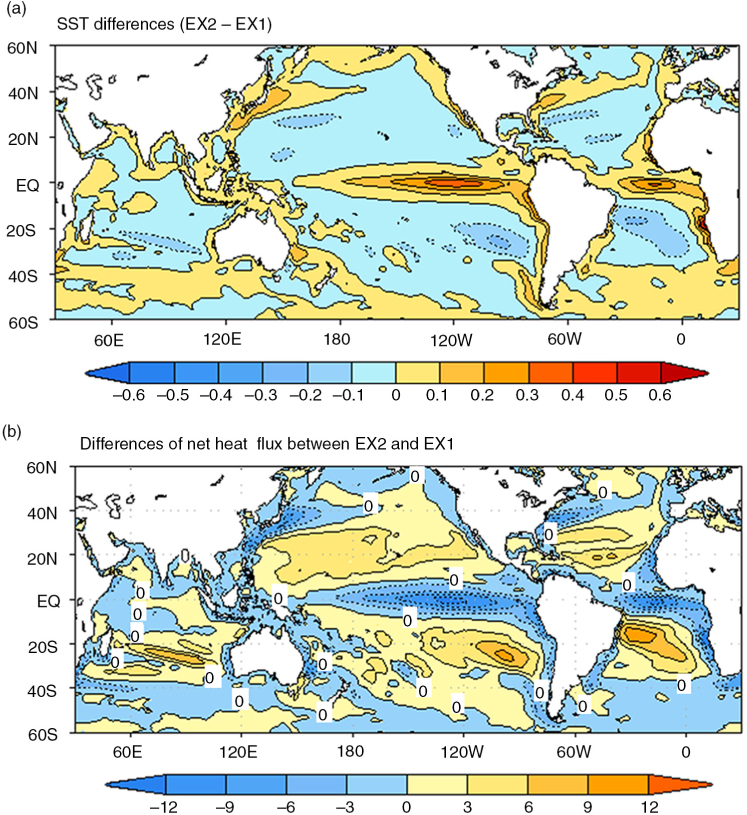
Fig. 4
The differences of annual mean SST (°C) (a) and net heat fluxes (w/m2) (b) between EX1 and EX2.
The differences in net heat flux between EX1 and EX2 (Fig. 4b) are almost opposite to their SST differences. This indicates that the model maintains its climatological SST by modulating the air-sea heat flux. In the tropical Pacific and Atlantic, EX2's net heat flux is almost 10 W m−2 less than EX1's. In the boundary current regions, such as Kuroshio, Gulf Stream, East Australian Current, Peru Current, Benguela Current, Agulhas Current, the net heat flux in EX2 is also significantly less than in EX1. However, EX2 has higher net heat flux than EX1 in the subtropical oceans, in particular along 20°S and 20°N. Our results are similar to those of Sweeney et al. (2005), who compared two different shortwave penetration schemes and used a strong 10-d SST restoration to seasonally varying observations, which is absent in our study.
4.1.3. Subsurface temperature.
Figure 5 shows the differences of the annual mean temperature between EX1 and EX2 at 150 m depth (Fig. 5a), averaged over the ocean's upper 300 m (Fig. 5b), along the equator and zonal mean temperature. Unlike the SST differences shown in Fig. 4a, the mean temperatures in EX2 at 150 m depth are higher than those in EX1 almost everywhere between 40°S and 40°N, since the shortwave diffusive attenuation coefficient in EX2 is smaller than that in EX1, resulting in deeper penetration of solar irradiance. Consequently, the subsurface in EX2 absorbs more heat than that in EX1. Broad-scale temperature differences (up to 1°C) occur along 20°N and 20°S. These differences are consistent with the large SWAD differences in these regions shown in Fig. 2d. The largest temperature difference (~1.5°C) is located around 25°S–30°S in the Indian Ocean at 150 m depth, due to both a large meridional temperature gradient and a significant SWAD difference in this area. The central equatorial Pacific also shows a large difference (~1°C), although the SWAD difference is only 4 m here. It is likely induced by the large east–west gradient of temperature in this region, as the cold water from the eastern Pacific is driven westward by the trade winds and meets the warm pool water from the west Pacific in the central Pacific. The temperatures averaged over the upper 300 m in EX2 are higher than those in EX1 in most areas (Fig. 5b). The spatial patterns shown in Fig. 5a and b are similar and largely coincide with the SWAD differences (Fig. 2d). This indicates that thermodynamics plays a major role in the temperature evolution of our simulations.
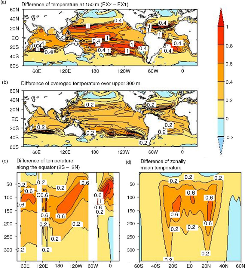
Fig. 5
The differences of annual mean temperature (°C) at 150 m (a); over upper 300-m oceans (b); along the equator (c) and zonal mean (d).
Along the equator (averaged from 2°S to 2°N), large differences occur in the thermocline region (Fig. 5c). The maximum value is about 0.6°C in the Pacific and Indian Oceans, and 1°C in the Atlantic. Figure 5d shows that the largest differences are located along 20°S, 20°N, and the equator, at depths between 100 and 200 m. The differences become less than 0.2°C near the sea surface and below 240-m depth where the solar radiation has been almost completely absorbed in both cases.
4.1.4. MLD and thermocline depth.
The difference in MLD between EX1 and EX2 is displayed in Fig. 6a. The mixed layer is defined as the depth at which the density of seawater is 0.03 kg m−3 greater than surface values. The MLD in EX2 is deeper than that in EX1 almost everywhere. Large MLD differences occur in the subtropical gyre. In the south-eastern Pacific, the MLD is up to 15 m deeper in EX2 than in EX1. Our results are similar to those of Sweeney et al. (2005). They mentioned that it was not clear whether or not there was a direct relationship between the increase in penetration depth and the increase in the MLD, since they used two different shortwave penetration schemes. However, all experiments in this study apply the same solar radiation scheme (Kara et al., 2005). The change in MLD clearly coincides with the SWAD differences (Fig. 2d). The larger SWAD produces a deeper mixed layer, since it allows the shortwave radiation to penetrate deeper, and heat the subsurface.
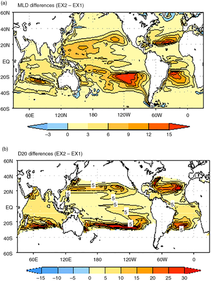
Fig. 6
The differences of mixed layer depth (a) and the 20° isotherm depth (b) between EX1 and EX2 (unit: m).
The differences of the 20°C isotherm depth (D20) are illustrated in Fig. 6b. The D20 is used as a proxy for thermocline depth in the tropical oceans. The D20 in EX2 is increased by about 5 m in the equatorial Pacific and Atlantic and about 30 m in the southern subtropical oceans relative to the D20 in EX1. The common feature of Fig. 6a and b is that the MLD and D20 in EX2 are larger than those in EX1 in the tropical oceans. The large differences which occur in the subtropical gyres are consistent with the SWAD differences. Note that the differences of SSH and steric height between EX1 and EX2 are consistent with the MLD or D20 differences (not shown). This indicates that the local SSH differences are associated with the temperature and density changes.
4.2. Analysis of ocean currents
4.2.1. Sea surface currents in cold tongue regions.
Figure 7 shows the differences in sea surface currents in the tropical Pacific (Fig. 7a) and Atlantic (Fig. 7b) between EX1 and EX2. EX2 produces an anomalously eastward and equatorward current near the equator relative to EX1. The anomalously eastward current represents a reduction of the westward current forced by the trade winds. The equatorward current indicates a weaker polarward meridional current in EX2, which results in a reduction of divergence near the equator and then weaken the cold upwelling. In general, the cold tongue extension is largely controlled by the trade winds and upwelling. Therefore, the EX2 has a deeper MLD shown in Fig. 6a, and warmer SSTs along the equator in the Pacific and Atlantic oceans. Murtugudde et al. (2002) also found that a spatially varied SWAD could reduce the cold tongue bias compared to a simulation in which a constant SWAD (17 m) was used. The spatially variable SWAD was greater than 17 m in most regions including the equatorial oceans.
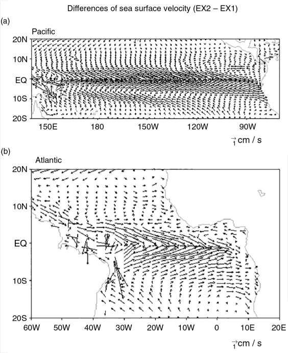
Fig. 7
Differences of sea surface velocity (cm/s) in the Pacific (a) and Atlantic (b) between EX1 and EX2.
4.2.2. Pacific equatorial undercurrent.
Figure 8 shows the annual mean zonal velocity along the equator over the Pacific Ocean in EX1 (Fig. 8a), and the difference between EX2 and EX1 (Fig. 8b). The surface flow is driven by trade winds from east to west, with a current reversal around 20–40 m depth; the eastward-flowing undercurrent is called the equatorial undercurrent (EUC). The core of the EUC reaches speeds of more than 100 cm s−1. Compared to EX1, the EUC in EX2 is reduced by a maximum of 7 cm s−1 at 160°W. The EUC is mainly forced by zonal pressure gradients, and it accelerates until the pressure gradient is balanced by frictional forces which tend to slow the current. To explore the cause of the reduction of the EUC in EX2 relative to EX1, we analyse the differences in the zonal pressure gradient. If the hydrostatic approximation is used, the approximated equations of motion for the EUC are
where u, v are the zonal and meridional velocity components, t is time, ρ density, p pressure, F x friction and g is acceleration due to gravity. The Coriolis force is denoted by f=2ω sinϕ , where ω is the angular velocity of the earth and ϕ is latitude. The Coriolis force can be ignored along the equator, but it keeps the EUC centred on the equator if the flow strays northward or southward.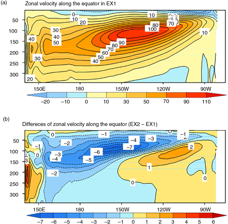
Fig. 8
(a) Annual mean zonal velocity (cm/s) along the equator in EX1 and the differences between EX1 and EX2 (b).
If we ignore the sea surface air pressure (since all experiments here use same COREv2 forcing), the pressure p can be integrated as
where ξ is SSH and z is depthThe pressure gradient in eq. (4) can be further expressed by accounting for eq. (6),
Therefore, the zonal pressure gradient is derived from the gradients of sea surface air pressure gradient, SSH and sea water density. All experiments here have same p a from external COREv2 forcings.The SSH (Fig. 9a) in the western Pacific is about 0.45 m higher than that in the eastern Pacific: this east–west SSH difference drives the EUC eastward. Although the SSH in EX2 is a little higher than that in EX1 everywhere, the zonal gradients of SSH (Fig. 9b) in both experiments are effectively the same. Therefore, we can exclude the SSH as a cause of the weaker EUC in EX2 than EX1. Figure 9c and d illustrate the difference of density and acceleration induced by the zonal density gradient between EX2 and EX1 along the equator section. The density in EX2 is smaller than that in EX1 in most regions due to its warmer temperature. The zonal acceleration (Fig. 9d) is weaker in EX2 than in EX1. The location of their large difference is between 100 and 200 m, and it is almost consistent with their EUC differences shown in Fig. 8b. Therefore, we can conclude that the greater shortwave penetration depth of EX2 produces warmer temperatures and reduces densities over the upper ocean, which then leads to a smaller zonal density gradient and consequently a slower EUC. Note that the difference of between EX2 and EX1 near sea surface is positive. This eastward acceleration anomaly will block the westward sea surface current driven by the trade winds and produces anomalously eastward current shown in Fig. 7.
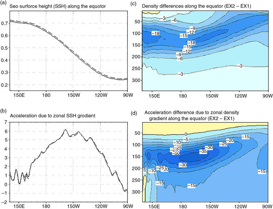
Fig. 9
(a) Annual mean sea surface height (m) (SSH) along the equator in EX1 (solid) and EX2 (dashed). (b) Same as (a) but with (10−7 m s−2). (c) The differences of annual mean density (10−2 kg m−3) along the equator between EX2 and EX1. (d) Same as (c) but with (10−7 m s−2).
4.2.3. Mean meridional current.
The large-scale meridional current is related to the mass and heat transport poleward from the tropics, and it is of critical importance to the global climate system. Figure 10 displays the averaged meridional current in the Pacific, Atlantic and the Indian Oceans, respectively, and their differences between EX1 and EX2. The velocities shown in Fig. 10a are almost antisymmetric about the equator. Meridional velocity initially decreases with depth, but reverses direction below 60 m. This character of velocity can be explained with classic Ekman theory. The Atlantic averaged meridional current (Fig. 10c) is similar to that in the Pacific, but the mean meridional current in the Indian Ocean has a different character (Fig. 10e). The southward current is much stronger than the northward current near the sea surface. The South Indian Ocean is strongly affected by the Indonesian Throughflow which carries the warm water from the western Pacific into the Indian Ocean (Hirst and Godfrey, 1993; Lee et al., 2002). The northward current is weaker than that in the Pacific and Atlantic, since the Indian Ocean currents are influenced by the Indian monsoon which reverses direction between the boreal winter and summer. In contrast, the equatorial Pacific and Atlantic meridional velocity is mostly controlled by the stable trade winds through the whole year.
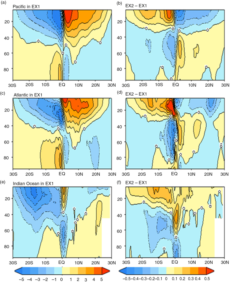
Fig. 10
(a) Annual mean meridional velocity zonally averaged in the Pacific (a), Atlantic (c) and the Indian Ocean (e) in EX1 in the left panel and their corresponding differences between EX1 and EX2 in (b)(d)(f) in the right panel (unit: cm/s).
Figure 10b, d and f display the differences in meridional velocity between EX1 and EX2. Poleward meridional velocities are generally reduced in EX2 compared with EX1, except the northward current in the Indian Ocean. In order to explain this phenomenon, the zonal-mean large-scale meridional motion can be represented by the following equation:
Here λ is longitude. λ 1 and λ 2 are the western and eastern boundaries of the ocean basin, respectively. For simplification, the item in eq. (4) can be omitted off the equator compared to the Coriolis force fv for the large-scale circulation. The meridional transport of water from low latitudes to the mid-latitudes is primarily driven by easterly winds. The wind stress at the sea surface is included in the F x term. F x also accounts for other small-scale frictions such as lateral viscosity. Note that the pressure gradient forces an opposing meridional transport pushing waters to the low latitudes. It indicates that the larger leads to lower meridional velocity under the condition of the same surface wind stress.According to eq. (7), can be expressed further as:
The item of integrated across the Pacific, Atlantic and Indian oceans is almost the same in EX2 as in EX1 (not shown). Figures 11 and 12 illustrate at the upper oceans between 30°S and 30°N in the three oceans. Figure 11 shows the total values integrated above 30 m and Fig. 12 displays the differences between EX2 and EX1 along the zonal section. The values of in EX2 are greater than those in EX1 everywhere near the sea surface, and the largest difference between EX2 and EX1 occurs in the subtropical regions near 25°S or 25°N. This indicates that the greater zonal pressure gradient induced by the larger density gradient in EX2 is the primary cause of the reduced meridional velocity. The differences of density gradient between EX1 and EX2 are largely caused by their temperature differences.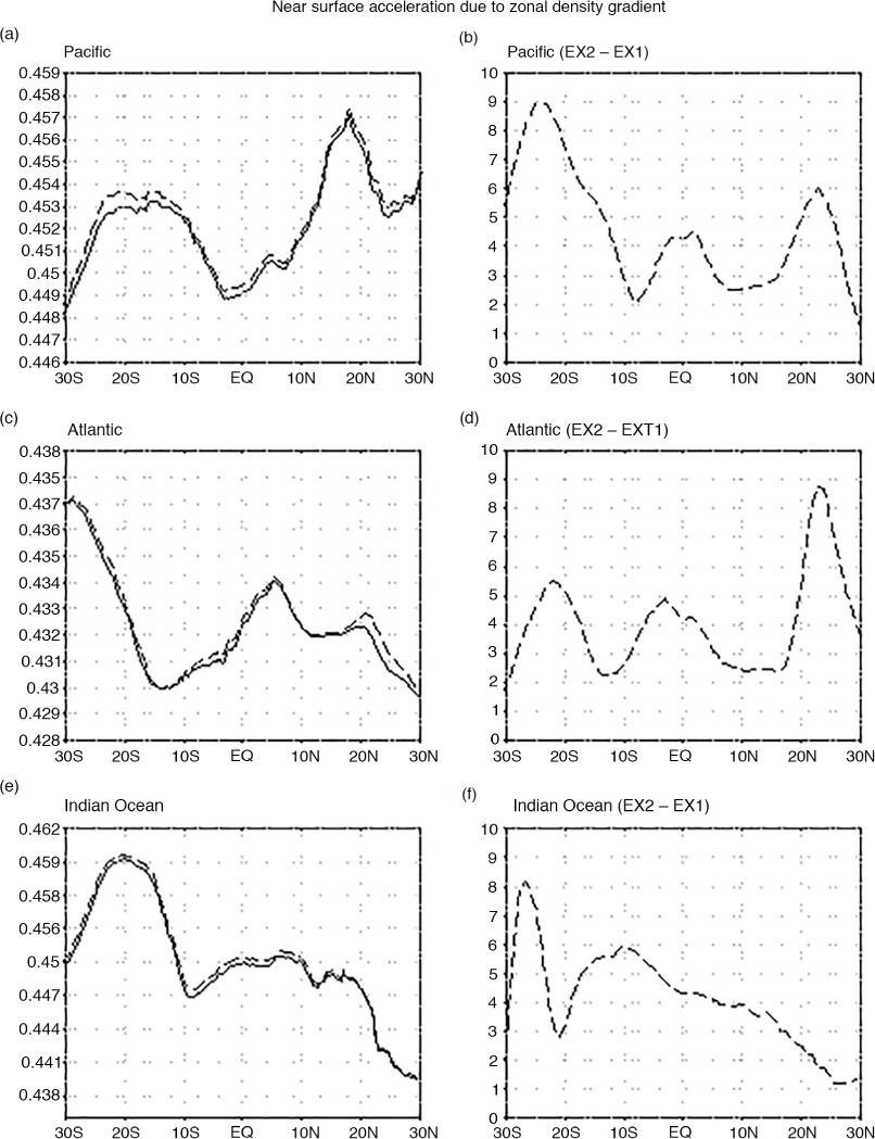
Fig. 11
Zonally averaged acceleration (10−3 m s−2) for EX1 and EX2 in the Pacific (a), Atlantic (c), Indian Ocean (e) and their differences (b, d, f, unit: 10−7 m s−2).
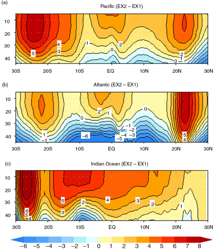
Fig. 12
The differences of zonally averaged acceleration (10−7 m s−2) between EX2 and EX1 in the Pacific (a), Atlantic (b), Indian Ocean (c).
Sweeney et al. (2005) compared two solar radiation schemes in their OGCM and found that their model with Ohlmann scheme (2003) produced a slowdown in meridional overturning between 30°S and 30°N in the Indo-Pacific basin relative to their model with the MA scheme (Morel and Antoine, 1994). They suggested that deeper mixed layers throughout the tropical oceans in the Ohlmann (2003) scheme is the main cause of a ~10% decrease in poleward transport of water in the surface layer. Our results show a reduction in meridional overturning in EX2 compared to EX1, due to a slower near-surface meridional velocity in EX2 induced by a larger density gradient. The density ρ in eq. (9) varies horizontally and vertically; however, the density ρ 0 in eq. (10) shown in the paper of Sweeney et al. (2005) is a constant.
4.3. Interannual variability
Figure 13a displays the differences of standard deviation of SST anomaly (SSTA, seasonal cycle is removed). Experiment EX2 has smaller SSTA standard deviations than EX1 almost everywhere, but the differences are generally small, about 10% of the corresponding SSTA. One of the reasons may be that the ocean model used here lacks any air-sea feedback. The interannual variability is mainly controlled by the external atmospheric forcing: the large SSTA standard deviation differences (up to 0.06°C) are located in the equatorial Pacific and Atlantic, areas of strong interannual variability. A weaker SSTA standard deviation is most likely due to a deeper MLD in EX2 than in EX1. Figure 13b shows the differences of standard deviation of temperature anomaly along the equator. EX2 has weaker interannual variability near the sea surface, but stronger variations in deeper oceans, since EX2 has a deeper thermocline.
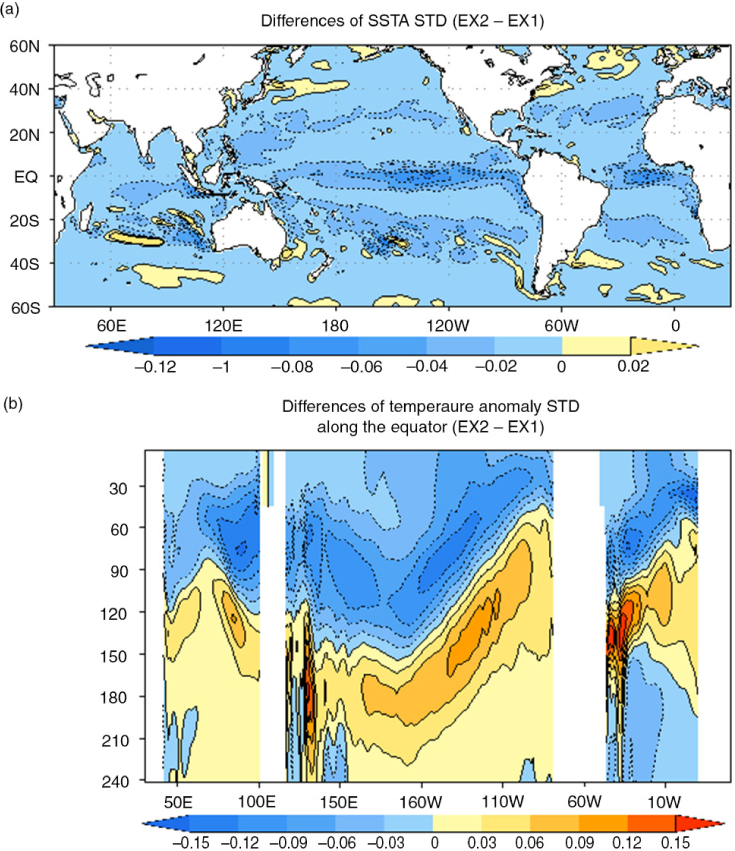
Fig. 13
Differences of SSTA standard deviation (a) and temperature anomaly standard deviation (b) along the equator between EX1 and EX2.
Figure 14 illustrates the time variations of SSTA (Fig. 14a) and D20 anomaly (Fig. 14c) in the Niño3.4 region in EX1 and the difference EX1 minus EX2 (Fig. 14b and d) from 1980 to 2007. EX2 tends to damp El Niño due to a deeper thermocline. This result is consistent with the conclusion of Anderson et al. (2009). The differences in Niño3.4 (5°N to 5°S, 170°W to 120°W) SSTA are generally less than 0.2°C, and are highly correlated with the SST anomaly (correlation coefficient of 0.78): a large ENSO event often produces a large SSTA difference between experiments. However, the differences of D20 anomaly between EX1 and EX2 do not coincide with the D20 anomalies so well (correlation coefficient of 0.46). The amplitudes of the D20 anomaly differences are less than 2 m.
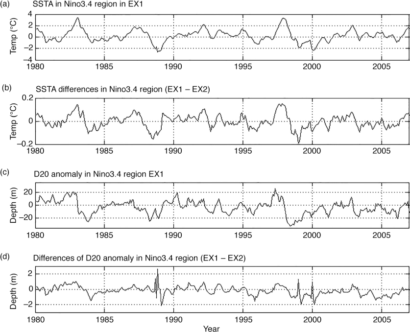
Fig. 14
The time evolutions of SSTA (a) and 20°C isotherm depth (c) in Ñino3.4 region and the differences between EX1 and EX2 (b, d) from 1980 to 2007 (unit: °C for temperature and m for D20).
5. Summary and discussions
In this study, three different SWADs estimated for PAR based on the K d(490) of SeaWiFS dataset have been applied in the ACCESS-OM model forced with the interannual COREv2 forcing from 1948 to 2007. Two estimates are based on the formulations of Morel et al. (2007) (experiments EX1 and EX2) and the third (experiment EX3) is simply the mean of these to estimates. In each case, the attenuation depth is spatially and seasonally varying. The attenuation depth in experiment EX2 is deeper than that in EX1 almost everywhere. The large differences (up to 10 m) occur in the oligotrophic gyres, whereas they become small in coastal areas with high chlorophyll concentrations. The difference in the eastern equatorial Pacific and Atlantic oceans is about 2 m.
Compared to experiment EX1, EX2 results in deeper penetration of solar radiation into the water column, which is expected to result in cooler SSTs and a warmer subsurface. This situation is the case for most of the ocean. However, in EX2, the surface waters are warmer in the equatorial Pacific and Atlantic oceans. Further analysis indicates that the warmer SST in EX2 is associated with that the EX2 produces anomalously eastward and equatorward surface currents near the equator and weakens the cold upwelling. It is consistent with the results from Murtugudde et al. (2002). Currently, most climate models have the problem of cold bias in the equatorial cold tongue regions. A deeper but realistic SWAD can partly solve this problem and then improve the El Niño simulation.
The temperature averaged over the upper 300 m in EX2 is warmer than EX1 between 40°S and 40°N. Large differences of temperature between EX1 and EX2 (up to 0.6°C) are located at depths of around 150 m along the equator, and at 20°S and 20°N. Experiment EX2 has a deeper MLD and D20 than EX1. The differences of MLD, D20 and averaged temperature over the upper oceans are largely consistent with SWAD differences between EX1 and EX2. A larger value of SWAD in the model produces a deeper MLD and D20, and higher temperatures at depths ranging from 30 to 300 m. These results are similar to previous studies such as Sweeney et al. (2005), Anderson et al. (2009) etc.
The SWAD value used in EX3 is the average of the SWAD values of EX1 and EX2. When considering the annual mean temperature error, the value from EX3 is almost exactly the same as the average of the same error statistic from EX1 and EX2. This suggests that the impact of different SWADs on the model temperature is largely linear.
Experiment EX2 produces a weaker Pacific EUC and meridional velocity than does EX1. This study firstly find that the reduced ocean current velocity is closely related to the acceleration derived from the zonal density gradient rather than the SSH. The force due to the zonal density gradient in the subsurface drives the EUC eastward along the equatorial Pacific. However, this force also blocks the poleward meridional transport off the equator. Our results show that EX2 has a weaker acceleration due to zonal density gradient in the subsurface along the equator. However, near the sea surface this acceleration, zonally averaged in the Pacific, Atlantic and Indian Oceans, is larger in EX2 than in EX1.
Experiment EX2 has a weaker interannual SST variability (standard deviation) than EX1, although the differences are relatively small. This is due to a deeper MLD and thermocline depth in EX2. The small differences are most likely amplified in the coupled atmosphere–ocean model due to air-sea feedbacks. Note that the SWAD used here does not have any interannual variability, whereas in reality the phytoplankton chlorophyll concentrations related to the SWAD do display strong interannual variability (Yoder and Kennelly, 2003). In the tropical Pacific, the phytoplankton chlorophyll concentrations are closely associated with the El Niño-Southern Oscillation; there may have a biological feedback mechanism (Park et al., 2011). A simple way of accounting for the interannual variability in the SWAD in a model is to construct an empirical model (Zhang et al., 2011). A biological and biogeochemistry model should be coupled in a climate model, and simulate the time-varying chlorophyll concentrations. These concentrations would be used to estimate the realistic SWAD, including its interannual variability.
Acknowledgements
This work was funded by the Australian Government Department of the Environment, the Bureau of Meteorology and CSIRO through the Australian Climate Change Science Programme. This work was supported by the NCI National Facility at the ANU.