

Fig. 1
HIRLAM analysis of sea/lake ice concentration (blue colour codes, in percentage), 850-hPa temperature (red lines, in °C) and the geopotential height at 850 hPa (black lines, in m) at the beginning (upper panel), middle (central panel) and at the end (lower panel) for the (left column) 2006 and (right column) 2012 events.

Fig. 2
Nested domains used in the simulation with some geographical references (a). The orography and land–sea border at domain 2 is shown in (b).
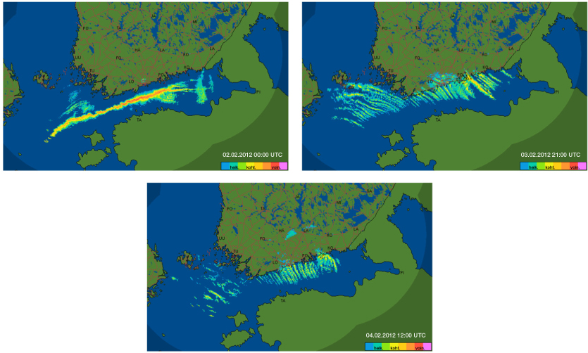
Fig. 3
Reflectivity images from the FMI weather–radar network on (upper panel) 2 at 0000 UTC, (middle panel) 3 February at 2100 UTC and (lower panel) 4 February 2006 at 1200 UTC. The colour scale indicate the reflectivity: blue and green colours are associated with low, yellow and orange with medium, and red and violet with high reflectivity.
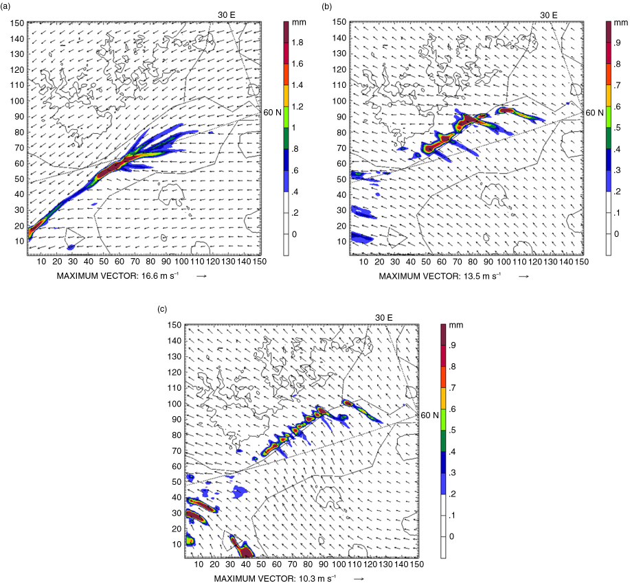
Fig. 4
Simulated 1-hour accumulated precipitation (colour contours) and surface wind field (arrows) in domain 2 on (a) 2 at 0000 UTC, (b) 3 at 2100 UTC, and (c) 4 February 2012 at 1200 UTC. Inland black lines are the 100 m orographic contour. The scale of the axes are in km.
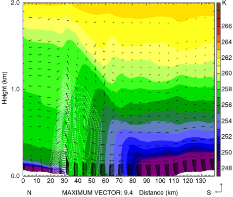
Fig. 5
Vertical cross-section along 25°E of the simulated potential temperature (colour contours), snow mixing ratio (white contours, maximum value 0.14 g kg−1) and the wind field (arrows) on 4 February 2012 at 0600 UTC. Estonian coast is on the right side, and Finnish coast is on the left.
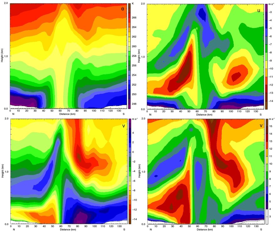
Fig. 6
Vertical cross-section along 25°E on 2 February 2012 at 0000 UTC of the potential temperature (θ), u wind component (u), v wind component (v), and the module of the horizontal wind speed (V). Estonian coast is on the right side, and Finnish coast is on the left.
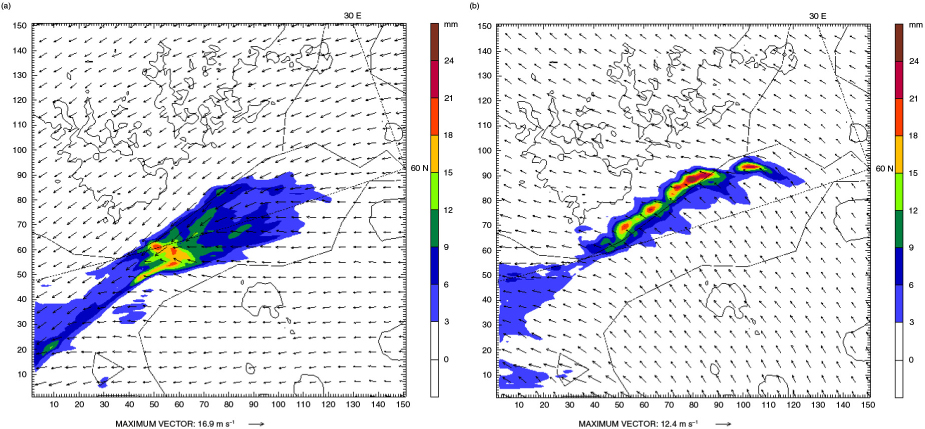
Fig. 7
Simulated 24-hour of accumulated precipitation (colour contours) and surface wind field (arrows) on (a) 3 February at 0000 UTC, and (b) 4 February 2012 at 0000 UTC. Inland black lines are the 100 m orographic contour. The scale of the axes is in km.

Fig. 8
Reflectivity images from the FMI weather–radar network on (upper panel) 18 at 0000 UTC, (middle panel) 19 at 1200 UTC and (lower panel) 20 January 2006 at 0000 UTC. The reflectivity scale is as in Fig. 3.

Fig. 9
Same as Fig. 4 on (a) 18 at 0000 UTC, (b) 19 at 0000 UTC, (c) 20 January 2006 at 0000 UTC and (d) 20 January 2006 at 0600 UTC. Inland black lines are the 100 m orographic contour. The scale of the axes is in km.
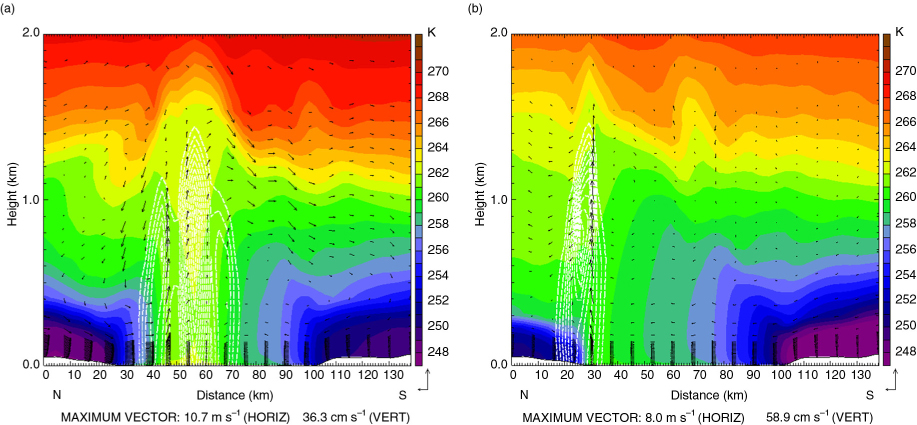
Fig. 10
Same as Fig. 5 on (a) 18 at 2200 UTC (Easterly regime) and (b) 20 January 2006 at 0400 UTC (Southerly regime). Maximum simulated snow mixing ratio is 0.17 g kg−1 in (a) and 0.15 g kg−1 in (b).

Fig. 11
Same as Fig. 6 on 18 January 2006 at 2200 UTC.
Table 1. Simulated values of the depth of the Estonian (H E) and Finnish (H F) cold-air outbreaks, maximum vertical wind velocity (w), the horizontal wind velocity (V LLJ) and the height (H LLJ) of the simulated low-level-jet in the Finnish (F) and Estonian (E) cells; and the inland-sea potential temperature difference (Δθ)
2006100010006016500–60019800–10001620124009009014400–50012700–80014