
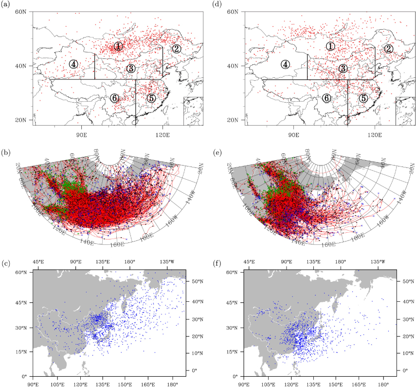
Fig. 1
Genesis regions (a) and (d), trajectories (b) and (e), and lysis locations (c) and (f) of cyclones (left panel) and anticyclones (right panel). The circled numbers correspond to ○1 Mongolia, ○2 Northeast China, ○3 North China, ○4 Northwest China, ○5 Central/Southeast China and ○6 Southwest China, divided by terrain and horizontal and vertical lines.
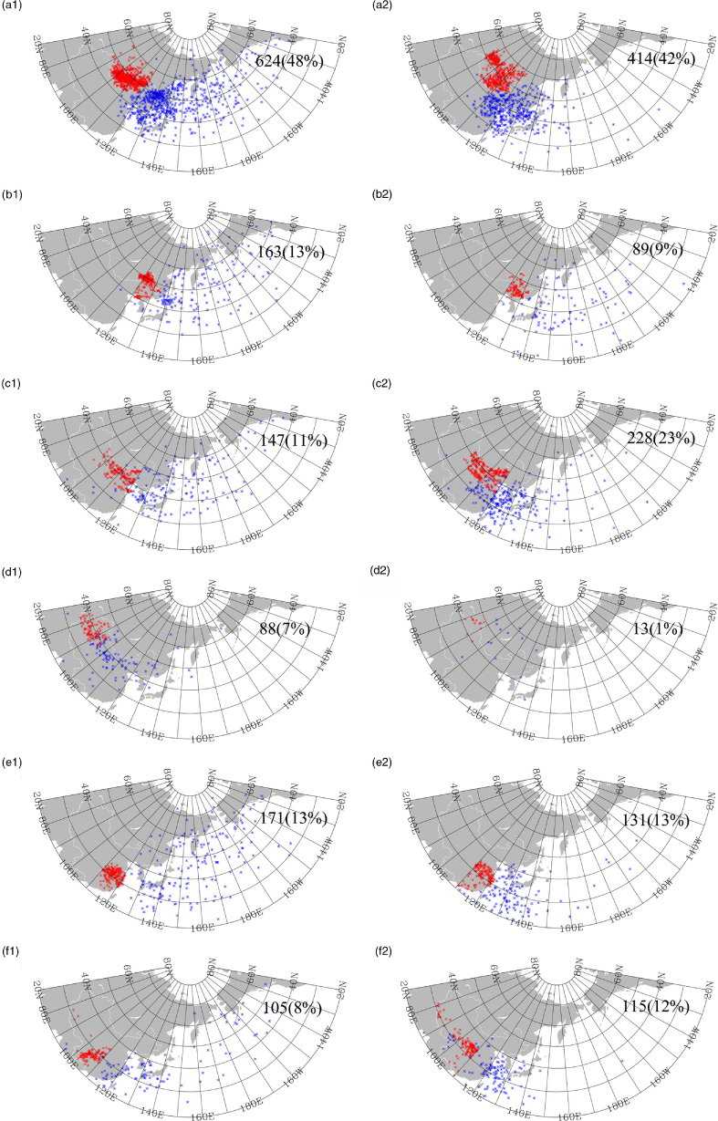
Fig. 2
Cyclone genesis (red dots) and lysis (blue dots) originating in ○1 Mongolia (a1), ○2 Northeast China (b1), ○3 North China (c1), ○4 Northwest China (d1), ○5 Central/Southeast China (e1) and ○6 Southwest China (f1). (a2)–(f2) The same except for the anticyclones. The number of cyclones or anticyclones and their corresponding percentages (in round brackets) are listed in the upper-right corners.
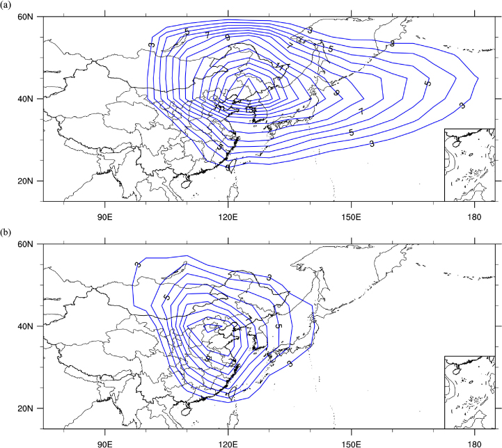
Fig. 3
Contours of CTCs (a) and ATCs (b) related to China (see text for explanation) per winter. The contour interval is one.
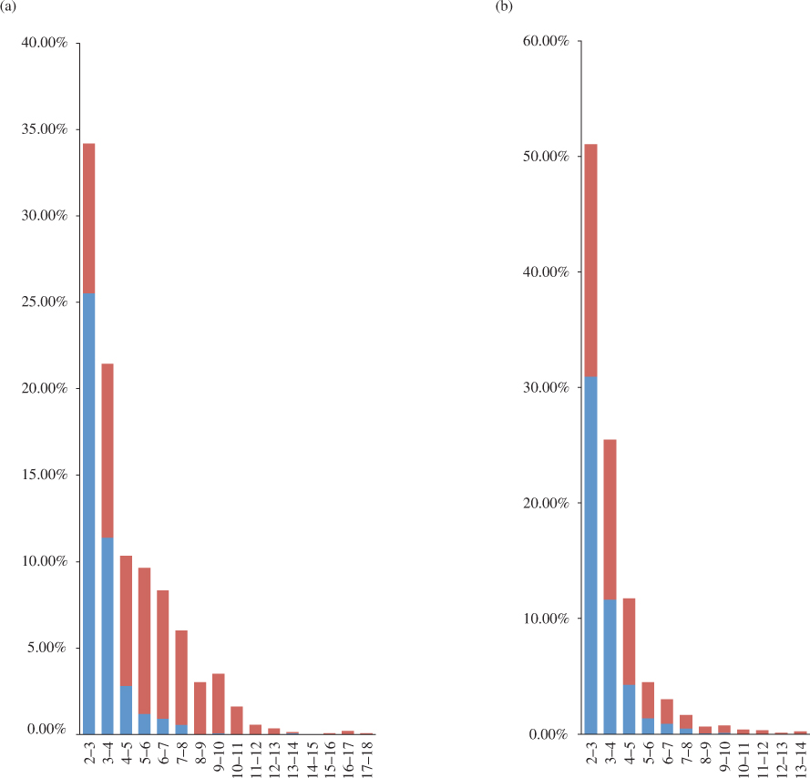
Fig. 4
Percentage of cyclones (a) and anticyclones (b) as a function of their lifespans. The red and blue column parts represent the stronger and weaker cyclones and anticyclones, respectively, in each lifespan range. The x-axis is in days. (Here, we define the stronger/weaker cyclones/anticyclones using their rank number. For example, all cyclones are sorted according to their maximum intensity; the median intensity is marked as the reference intensity. Cyclones in which the maximum intensity is greater (less) than the reference intensity are treated as stronger (weaker) cyclones. This same procedure is also used for anticyclones.)
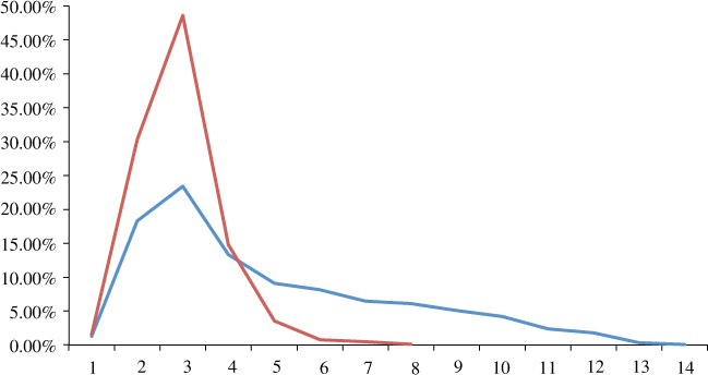
Fig. 5
Percentage of cyclones (blue curve) and anticyclones (red curve) as a function of their absolute maximum intensities. The x-axis is in 10−5 s−1.
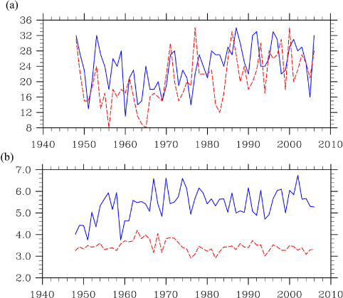
Fig. 6
Interannual variations in number (a) and average maximum intensity (b) of cyclones (blue solid curves) and anticyclones (red dashed lines) affecting China.
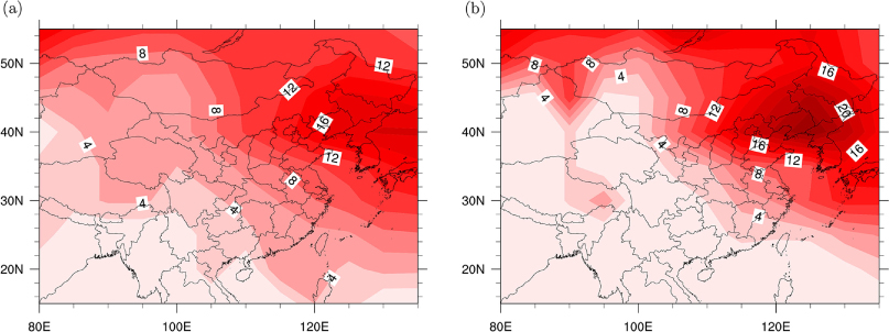
Fig. 7
Climatological mean (a) and variance (b) of the transit count for wintertime cyclones from 1948 to 2007. The contour intervals are two.
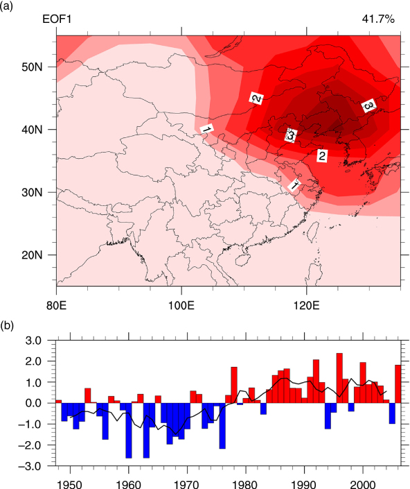
Fig. 8
EOF1 of CTCs for the 1948–2007 period in East Asia: (a) spatial mode/loading field and (b) normalised time series (bars). The black curve is the filtered time series after a 5-yr running mean. The contour interval is 0.5 in (a).

Fig. 9
Climatological mean (a) and variance (b) of the transit count for wintertime anticyclones from 1948–2007. The contour intervals are two in (a) and five in (b).
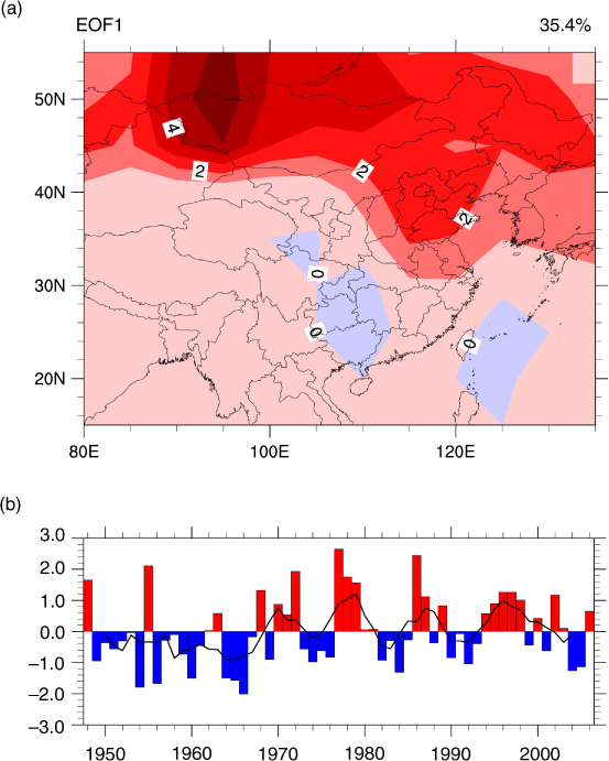
Fig. 10
EOF1 of ACTs for the 1948–2007 period in East Asia: (a) spatial mode/loading field and (b) normalised time series (bars). The black curve is the filtered time series after a 5-yr running mean. The contour interval is one in (a).
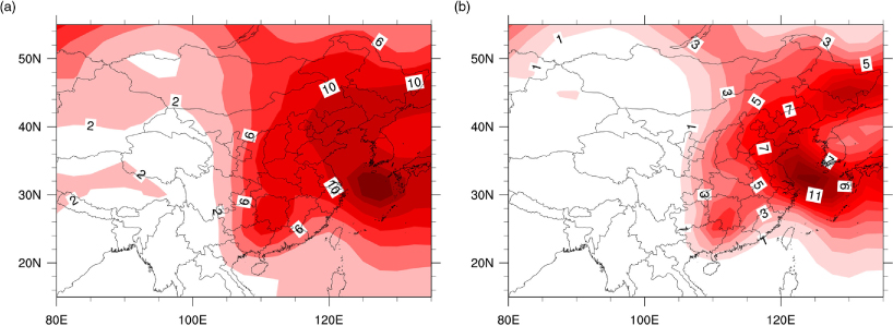
Fig. 11
Climatological mean (a) and variance (b) of the two- to seven-day bandpass-filtered 850-hPa meridional wind variance for the 1948–2007 period. The contour intervals are 2 m2/s2 in (a) and 1 m4/s4 in (b).
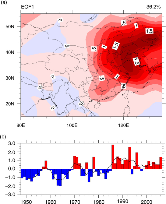
Fig. 12
EOF1 of the two-to seven-day bandpass-filtered 850-hPa meridional wind variance for the 1948–2007 period in East Asia: (a) spatial mode/loading field and (b) normalised time series (bars). The black curve is the filtered time series after a 5-yr running mean. The contour interval is 0.25 m2/s2 in (a).
Table 1. Correlation between the first mode of variability for storm tracks (ST) at 850 hPa and the leading modes of variability for the CTC, ATC and C&ATC
ST-850 hPa PC-10.62**0.28*0.58**

Fig. 13
Climatological mean (a) and variance (b) of the wintertime zonal mean (80–120°E) zonal wind for the 1948–2007 period. The contour intervals are 5 m/s in (a) and 2 m2/s2 in (b).

Fig. 14
Spatial mode/loading field of EOF1 (a) and EOF2 (c) for the ZMZWs (80–120°E) in the wintertime East Asia troposphere (100–1000 hPa and 15–55°N) for the 1948–2007 period. The contour intervals are 0.25 m/s. The corresponding normalised time series (bars) are also shown (b) and (d). The black curve is the filtered time series after a year running mean.
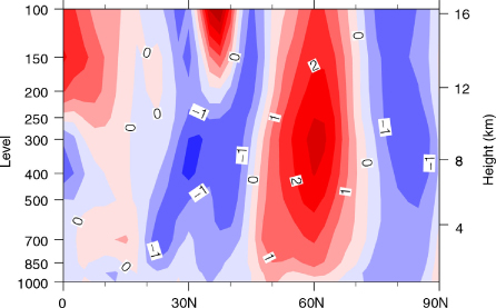
Fig. 15
Composite differential map between 1984–2003 and 1964–1983 for the ZMZW (80–120°E). The contour interval is 0.5 m/s.