
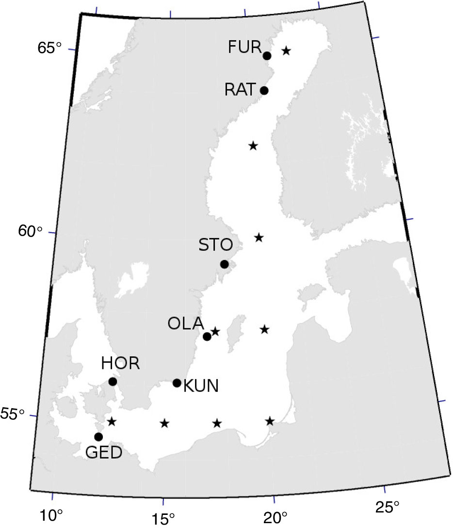
Fig. 1.
Map with the location of analyzed tide gauges (•) and reanalysis gridpoints (★).
{ label needed for table-wrap[@id='UT0001'] }
Table 1. Analysed daily tide gauge records
Gedser (GED)11.9354.574.09Hornbæk (HOR)12.4756.103.90Kungsholmsfort (KUN)15.5856.100.54Ölands Norra Udde (OLA)17.0157.364.01Stockholm (STO)18.8059.311.11Ratan (RAT)20.9264.000Furuögrund (FUR)21.2364.920.22
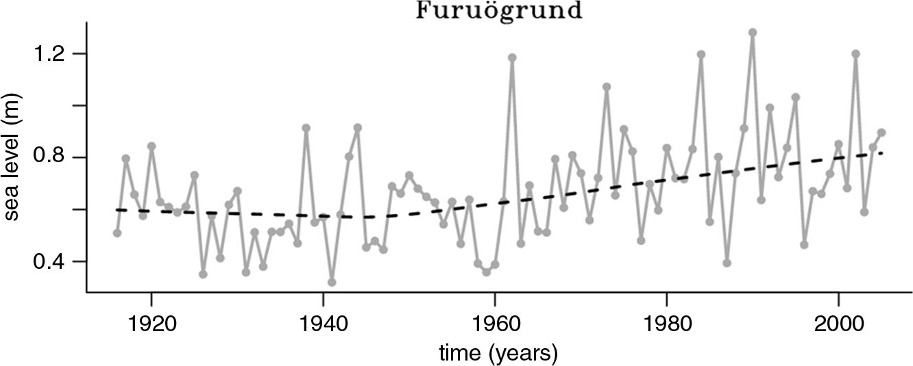
Fig. 2.
Sequence of annual maxima for Furuögrund (solid) and corresponding lowess smooth (dashed).
{ label needed for table-wrap[@id='UT0002'] }
Table 2. Likelihood ratio test (Q) for the null hypothesis (H 0) of a Gumbel non-stationary model (ξ=0) and for a stationary model (β 1=0)
Gedser3.560.18Hornbæk3.300.72Kungsholmsfort0.065.36Ölands Norra Udde2.130.03Stockholm–3.49Ratan4.124.94Furuögrund1.4613.09
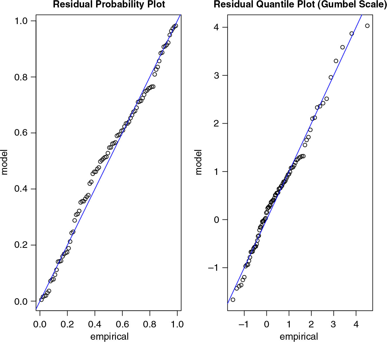
Fig. 3.
Diagnostics plots: probability plot (left) and quantile-quantile plot (right) for the Furuögrund model.
Table 3. Maximum likelihood estimates for µ, σ and ξ of the selected models (standard errors in parentheses)
Gedser665.61 (15.66)140.66 (10.91)0Hornbæk696.69 (16.22)145.46 (11.43)0Kungsholmsfort428.61 (18.86)0.87 (0.35)91.61 (8.17)0Ölands Norra Udde485.07 (13.28)119.20 (9.55)0Stockholm384.74 (9.87)89.09 (7.54)0Ratan466.52 (37.38)1.87 (0.76)159.61 (13.20)−154.99 (70.64)Furuögrund467.10 (34.32)2.56 (0.66)154.42 (12.60)0
Table 4. Return levels (m) for 10, 25, 50 and 100 yr
Station10 yr25 yr50 yr100 yr
Gedser0.981.121.211.31Hornbæk1.021.161.261.37Kungsholmsfort0.640.730.790.86Ölands Norra Udde0.750.870.951.03Stockholm0.560.670.730.79Ratan0.770.870.941.00Furuögrund0.830.981.091.20
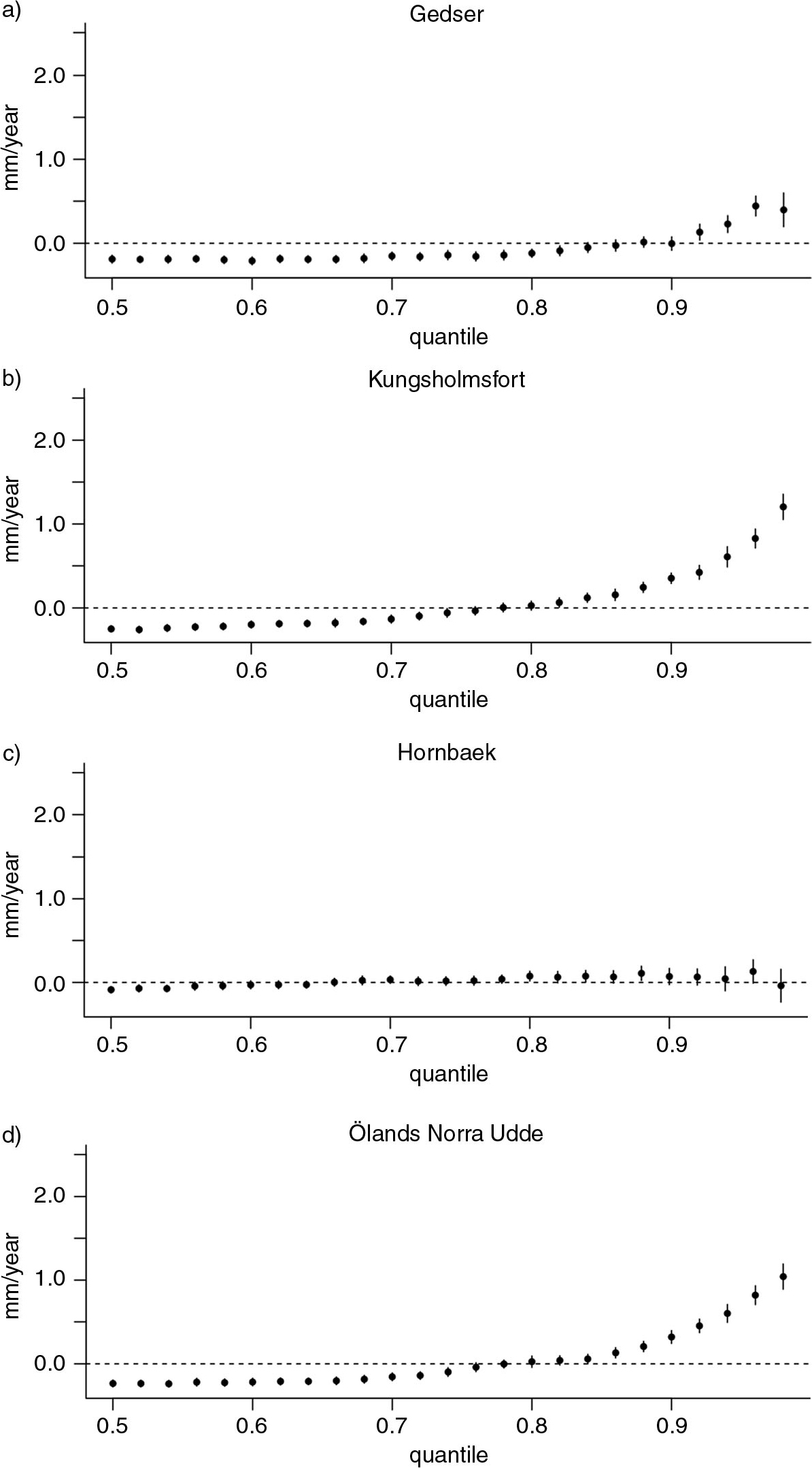
Fig. 4.
(Continued)
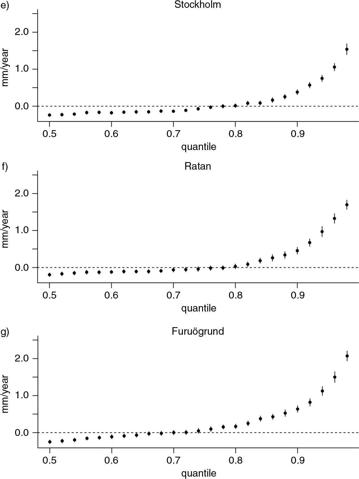
Fig. 4.
Quantile slopes (points) and corresponding standard errors (vertical error bars). The horizontal dashed line denotes the mean (0 mm/yr) trend.
Table 5. Quantile regression trends (standard errors in parentheses) and corresponding bootstrap estimates (ensemble median and IQR) for quantile 0.98
Gedser0.40* (0.22)0.40 (0.05)Hornbæk−0.04 (0.18)−0.04 (0.02)Kungsholmsfort1.20* (0.14)1.23 (0.06)Ölands NorraUdde1.04* (0.13)1.05 (0.07)Stockholm1.54* (0.15)1.55 (0.07)Ratan1.70* (0.12)1.74 (0.08)Furuögrund2.07* (0.14)2.10 (0.08)
Table 6. Likelihood ratio test (Q) for the null hypothesis (H 0) of a stationary GEV model (β 1=0) for the atmospheric data
12.5°E 55.0°N3.130.822.010.6815.0°E 55.0°N2.590.96––17.5°E 55.0°N4.201.2220.5412.6520.0°E 55.0°N2.331.4916.3311.8717.5°E 57.5°N4.920.830.172.820.0°E 57.5°N2.271.0805.7620.0°E 60.0°N1.740.300.070.1620.0°E 62.5°N1.780.441.610.2922.5°E 65.0°N0.830.9815.755.70
Table 7. Maximum likelihood estimates for the slope (β 1) of the non-stationary GEV models (standard errors in parentheses)
12.5°E 55.0°N–––15.0°E 55.0°N–––17.5°E 55.0°N0.28 (0.13)0.62 (0.0020)0.31 (0.0021)20.0°E 55.0°N–0.54 (0.0020)0.32 (0.0036)17.5°E 57.5°N0.22 (0.10)––20.0°E 57.5°N––0.31 (0.0020)20.0°E 60.0°N–––20.0°E 62.5°N–––22.5°E 65.0°N–0.30 (0.0020)0.21 (0.0045)
Table 8. Quantile regression trends (standard errors in parentheses) for quantile 0.98
12.5°E 55.0°N0.17 (0.039)*0.035 (0.012)*0.28 (0.054)*0.076 (0.046)15.0°E 55.0°N0.14 (0.041)*0.042 (0.012)*0.42 (0.054)*0.081 (0.040)*17.5°E 55.0°N0.16 (0.041)*0.039 (0.011)*0.42 (0.059)*0.20 (0.038)*20.0°E 55.0°N0.16 (0.040)*0.048 (0.011)*0.33 (0.055)*0.21 (0.037)*17.5°E 57.5°N0.20 (0.036)*0.034 (0.012)*0.030 (0.058)−0.028 (0.050)20.0°E 57.5°N0.19 (0.035)*0.030 (0.013)*0.023 (0.063)−0.076 (0.052)20.0°E 60.0°N0.19 (0.031)*0.0067 (0.013)0.11 (0.051)*−0.0002 (0.051)20.0°E 62.5°N0.078 (0.037)*−0.011 (0.013)0.093 (0.045)*0.032 (0.043)22.5°E 65.0°N0.12 (0.028)*−0.025 (0.016)0.18 (0.051)*0.083 (0.04)*