
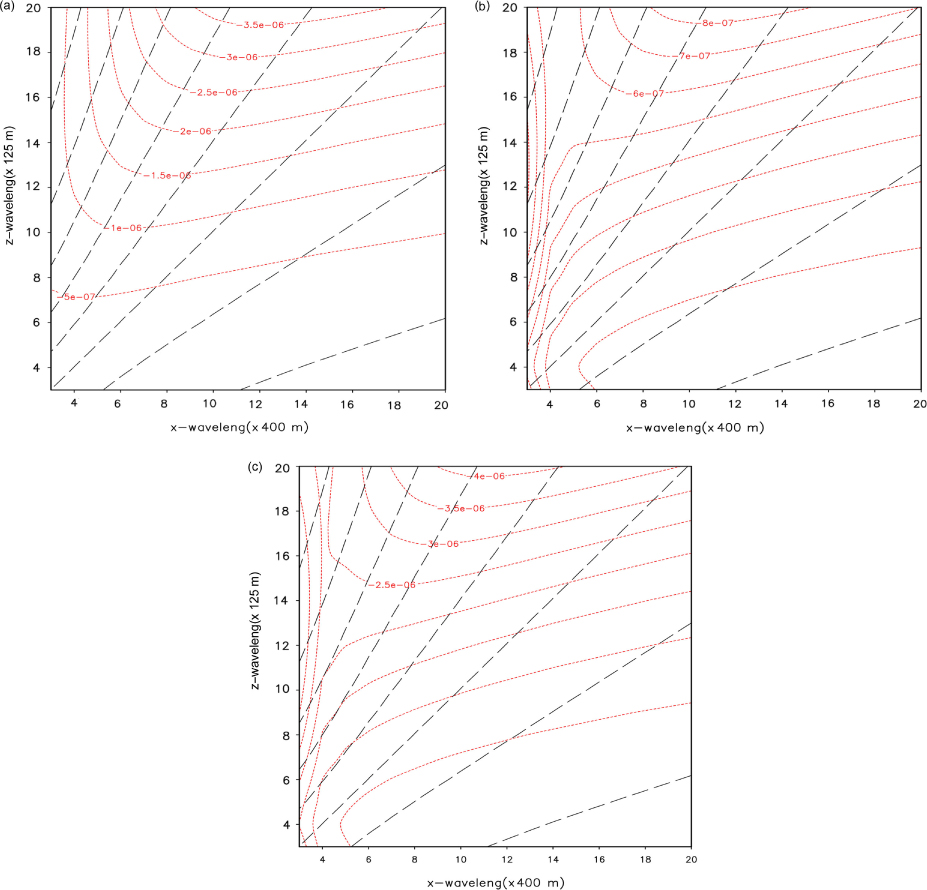
Fig. 1
Frequency of gravity wave with g=10 m s−2, C=300 m s−1, Δx=400 m, Δz=125 m, and S o =1.0−5 m−1: (a) ω δ=16 (Δt=1.59 s, dash) and ω δ=16 − σ g (dot); (b) ω˜ δ=4 (Δt=1.68 s) and ω˜ δ=4 − σ g ; and (c) ω˜ δ=16 (Δt=3.18 s) and .
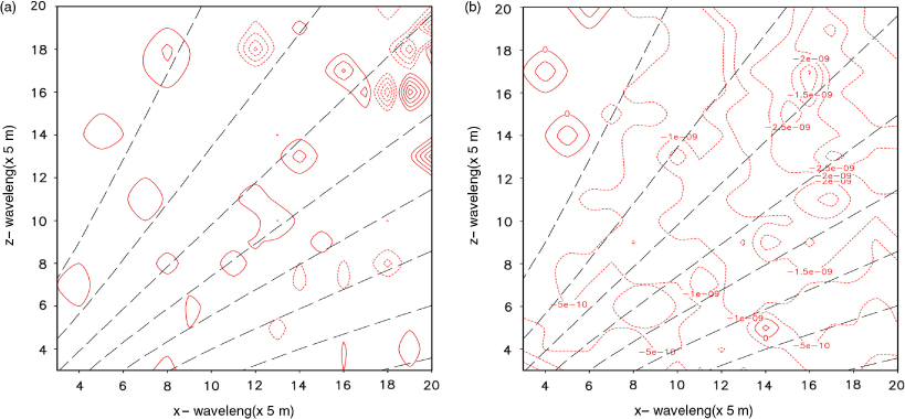
Fig. 2
(a) Frequency of ω δ=16 (Δt=4.71×10⁻² s, dash) from 0.002 (dashed line at right-bottom corner) to 0.009 s−1 with interval of .001 s −1, and ω δ=16−σ g (dot) from –2.5×10⁻⁸ to 2.0×10⁻⁸ s−1 with interval of 1.0×10⁻⁹ s−1; (b) δ=16 (Δt=9.42×10⁻² s and smoothing), and from −3.5×10⁻⁹ to 5.0×10⁻¹⁰ s−1 with interval of 5.0×10⁻¹⁰ s−1.

Fig. 3
(a) Initial x-component wind for Kelvin-Helmholtz instability for Section 4.1–4.2; (b) initial background θ 0 (solid) and perturbation θ’ (dot) for large-scale waves discussed in Section 4.1.
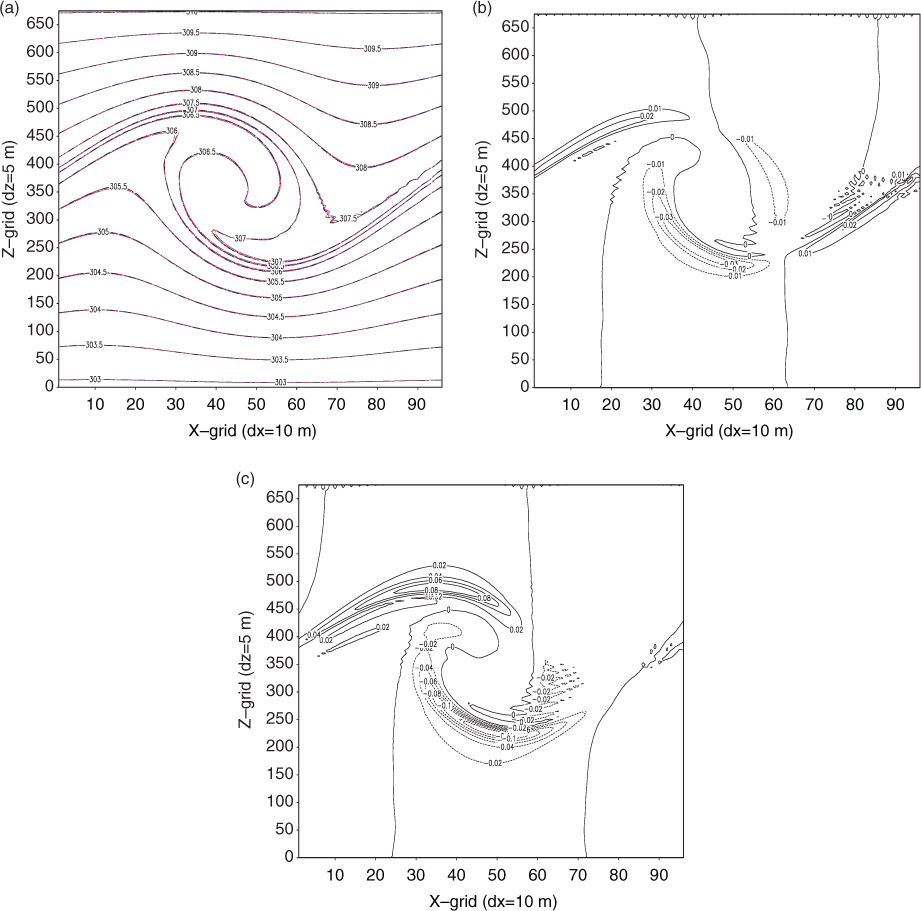
Fig. 4
Simulations for large-scale Kelvin-Helmholtz instability at t=320 s with Δtb=0.4 s from (a) θ FB (δ=1, Δts=0.01 s); MFB (δ=16, Δts=0.04 s); MFBS(δ=4, Δts=0.04 s); MFBS (δ=16, Δts=0.08 s), and HE–VI (Δts=0.02 s); (b) θ MFBS (δ=4, Δts=0.04 s) − θ FB (Δts=0.01 s), contours from –0.03 to 0.03 K with interval of 0.01 K; (c) θ MFBS (δ=16, Δts=0.08 s) −θ FB (Δts=0.01 s), contours from –0.12 to 0.08 K with interval of 0.02 K.
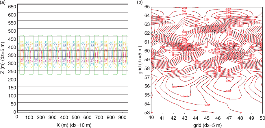
Fig. 5
As above but for small-scale Kelvin-Helmholz instability simulation (a) initial background θ 0 (solid) and perturbation θ’ (dash); (b) simulated θ’ at t=240 s from FB (δ=1, Δts=0.005 s, red solid), and MFBS (δ=16, Δts=0.04 s, blue dash). Contour interval is 0.002 K.
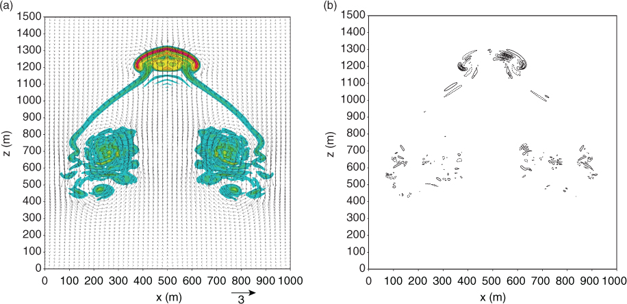
Fig. 6
Simulations at t=18 min: (a) velocity V MFBS and θ MFBS (δ=16, Δts=0.06 s, black contours), and θ FB (Δts=0.008 s, colour shaded), contours from −0.15 to 0.6 K; and (b) θ MFBS (δ=16, Δts=0.06 s) − θ FB (Δts=0.008 s), contours from −0.03 to 0.04 K.
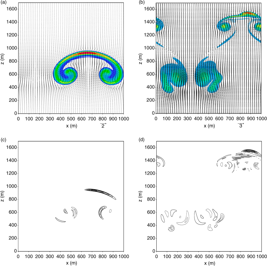
Fig. 7
(a) Simulated velocity perturbation V’ MFBS and θ MFBS (δ=16, Δts=0.06 s) at t=12 min, (b) same as (a) but at t=24 min, (c) θ MFBS−θ FB (Δts=0.008 s) at t=12 min, contours from −0.004 to 0.006 with interval of 0.001, and (d) θ MFBS−θ FB at t=24, contours from −0.015 to 0.02 K with interval of 0.005 K.

Fig. 8
Simulations at t=9000 s with Δx=400 m, Δz=125 m and Δtb=10 s: (a) w δ=1 (Δts=0.25 s, black dotted); w δ=16 (Δts=1.0 s, red short-dash); w MFBS (Δts=2.0 s, δ=16, green long-dash); and w HE–VI (Δts=1.0 s, blue long-dash, short dash); (b) w δ=16−w δ=1 (red dash) and w MFBS−w δ=1 (black solid); and (c) w HE–VI –w δ=1 (red dash) and w MFBS (δ=16, Δts=2.0 s)–w δ=1 (black solid), the contour interval is 0.02 m s−1.