
1. Introduction
The eigenvalues and non-linear simulations of the non-hydrostatic model (NH) using the conventional forward–backward scheme (FB) (Mesinger and Arakawa, 1976; Sun, 1980, 1984), the horizontal explicit and vertical implicit scheme (HE–VI) (Klemp and Wilhelmson, 1978; Saito, 2007) and the modified non-hydrostatic model (MNH) have been discussed in Sun et al. (2012), hereafter referred to as Part I. The MNH is designed to suppress high-frequency acoustic waves by multiplying the left-hand side of the continuity equation by a parameter δ, where 16≥δ≥4. When δ=1, the MNH and NH are identical. Since the FB is applied to solve NH and MNH, they called their approach a modified forward–backward scheme (MFB) for δ>1; MFB is the same as the conventional FB when δ=1.
In Part I, frequency of acoustic waves is greatly reduced by the MFB, but much less so for gravity waves. Also, the MFB is more accurate for smaller values of δ or finer space intervals. The non-linear non-hydrostatic Cloud Resolving Storm Simulator (CReSS; Tsuboki and Sakakibara, 2002, 2007) showed that Kelvin-Helmholtz instabilities, thermal bubbles and mountain waves simulated by a conventional FB can be reproduced using an MFB with a time interval four times longer. It was also found that the shortest waves (i.e. 2Δx and/or 2Δz) require the shortest time interval according to the Courant-Fredrich-Lewy (CFL) criterion. Since the accuracy of gravity waves decreases as δ increases, it seems preferable to filter 2Δx and 2Δz waves rather than increase the value of δ. Hence, in addition to multiplying δ (δ≤16 in Part I) in the continuity equation of MNH, we propose to apply smoothing on the right hand of the continuity equation to damp the short waves. We refer to the resulting model as the modified non-hydrostatic model with smoothing (MNHS). The eigenvalue and non-linear model simulations show that, for the same accuracy, MNHS allows twice the time interval of MNH. It is also noted that other numerical schemes, for example: the modified leapfrog scheme (Sun and Sun, 2011) and/or the new semi-implicit scheme (Sun, 2011) can be applied to the wave-related terms of the MNHS to achieve the same efficiency as discussed in this paper.
2. Basic and linearised equations
The 2-D non-hydrostatic equations for the dry atmosphere can be written as:
where u and w are the x and z components of wind; p is pressure; θ is potential temperature; T is temperature; ρ is density; R is gas constant; C p is specific heat at constant pressure; D u and D w are momentum diffusions along the x and z directions; D θ is the heat diffusion. The linearised equations become:
where primes indicate deviations from the basic state variables (with subscript ‘0’), which are functions of height only, and The basic state wind is assumed to be zero. In Part I, δ>1 was introduced in the continuity equation in order to filter high-frequency acoustic waves. Following the procedure in Part I, eqs. (7)–(11) can be formulated as:
The linearised equations show that the 2Δx and/or 2Δz waves require the shortest Δt to satisfy the CFL criterion. Therefore, to relax the time step limitation, we apply smoothing on the right-hand side of eq. (15). Thus, eq. (15) is replaced by
where
and
is the two-dimensionally smoothed version of f. Where k and m are the wave numbers in the x and z directions, respectively. Equation (15) can now be written
and
Equations (17) and (18) indicate that 2Δx and 2Δz waves are removed from convergence/divergence. The 3Δx and 3Δz waves, which can create non-linear instability, are also significantly reduced by the second-order smoothing. The effect of smoothing decreases with increasing wavelength. The value of cos(kΔx/2)=0.809 for a 5Δx-wave seems to imply that the errors can be quite large for 5Δx and shorter waves according to eq. (17). However, linear stability analysis shows that smoothing does not significantly affect the results for wavelengths longer than 3Δx. Non-linear model simulations also reveal that the accuracy of the MNH (without smoothing) is comparable to that of the MNHS (with smooth) for the same value of δ, even when the time interval for MHNS is twice that for MNH. In Section 3, we will show the eigenvalues of the MNH, MNHS and HE–VI models, as well as their comparisons with , the eigenvalue of gravity waves derived from the differential in time and difference in space [eq. (2. 18) in Part I]:
where and
3. Eigenvalue of finite difference equations
The solutions of eqs. (12)–(15) can be assumed:
where ˜λ is the complex amplification factor.
3.1. The finite difference form and eigenvalues of the modified FB
Following Part I, the Arakawa C grids are used in the eigenvalue analysis; a forward in time scheme is applied to the momentum fields and a backward to the pressure and temperature, producing finite difference equations for eqs. (12)–(15),
The eigenvalues for the modified forward–backward scheme with smoothing (MFBS) can now be determined from
orWithout smoothing, eqs. (25) and (26) are identical to eq. (3.6) of Part I, which consists of two acoustic waves and two gravity waves. Let us define:
The amplification ∣˜λ∣ factor is then unity if Δt≤Δ˜tδ . In that case, the frequency ˜ωδ is defined by
and
Without smoothing, the values of ˜λ, ˜ωδ , and Δ˜tδ of eqs. (25)–(29) are also equal to λ δ , ω δ , and Δt δ of MFB discussed in Part I.
With g=10 m s−2, C=300 m s−1, Δx=400 m, Δz=125 m, S o =1.0×1.0−5 m−1 and δ=16, we obtain Δt δ=16=1.59 s according to eq. (27) without smoothing. Figure 1 shows that: (a) the frequency of ω δ=16 (from 0.002 near the right-bottom corner to 0.009 s −1 with interval of 0.001 s−1) and ω δ=16−σ g (from −3.5×10⁻⁶ to −5.0×10⁻⁷ s−1); (b) and (from –8×10⁻⁷ to −1.0×10⁻⁷ s−1); and (c) and (from −4.×10−6 to −5.0×10⁻⁷ s−1). Smoothing of the continuity equation creates a large error for the 2Δx (and/or 2Δz) waves in Fig. 1b and c. Because those short-waves cannot be calculated accurately using the finite difference schemes, the eigenvalues of the unwanted 2Δx and 2Δz waves are not presented here. The error associated with smoothing decreases drastically with increasing wavelength. The errors for 3Δx waves, of –8×10⁻⁷ s−1 in Fig. 1b and −3.5×10⁻⁶ s−1 in Fig. 1c, are comparable with the errors at longer wavelengths. With approximately the same Δt (~1.6 s), the maximum value of (=∣8×10⁻⁷∣ s−1) is much less than the maximum of (=∣3.5×10⁻⁶∣ s−1). The error of (=∣4×10⁻⁶∣ s−1) is also comparable with the error of ω δ=16(=∣3.5×10⁻⁶∣ s−1), where the time interval used for (Δt=3.08s) is twice that for ω δ=16(Δt=1.59s).
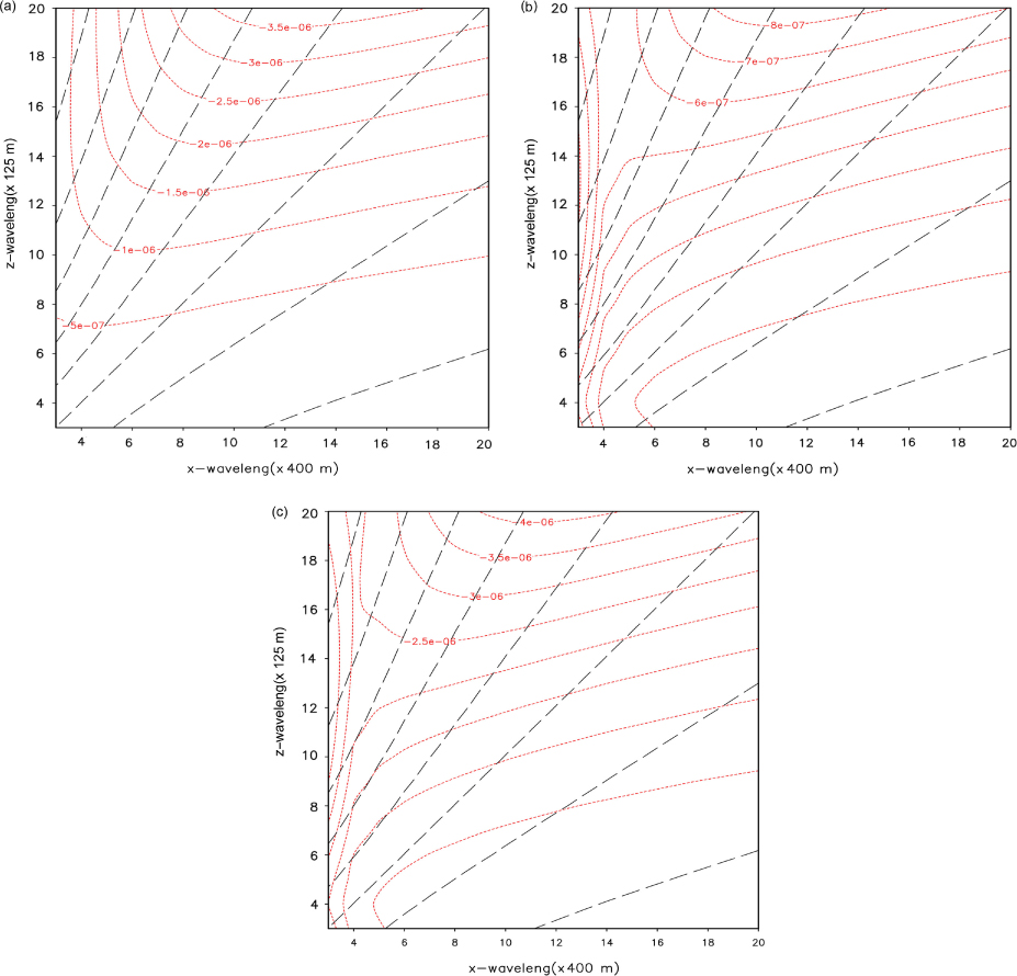
Fig. 1
Frequency of gravity wave with g=10 m s−2, C=300 m s−1, Δx=400 m, Δz=125 m, and S o =1.0−5 m−1: (a) ω δ=16 (Δt=1.59 s, dash) and ω δ=16 − σ g (dot); (b) ω˜ δ=4 (Δt=1.68 s) and ω˜ δ=4 − σ g ; and (c) ω˜ δ=16 (Δt=3.18 s) and .
When the basic state remains the same and Δx=5 m and Δz=5 m, Δt δ=16=4.71×10⁻² s according to eq. (27) without smoothing. Figure 2a shows that the frequency of ω δ=16(Δt=4.71×10⁻² s) is from 0.002 to 0.009 s−1, and ω δ=16−σ g is from −2.5×10⁻⁸ to 2.0×10⁻⁸ s−1. With smoothing, δ=16, and Δt=9.42×10⁻² s, and (from −3.5×10⁻⁹ to 5.0×10⁻¹⁰ s−1) are shown in Fig. 2b. The accuracy of is better than ω δ=16, which indicates that smoothing of the continuity equation does not deteriorate the accuracy of eigenvalues in the fine resolution case. Part I showed that the MNH (with δ=16) is capable of reproducing the FB results with a time interval four times longer. When spatial smoothing is added to MNH, the allowable time interval becomes eight times that of FB, according to linearised equations, without significantly reducing the accuracy. Note also that Part I showed that in a fine-resolution model with small aspect ratio, the MFB is more accurate and efficient than HE–VI.
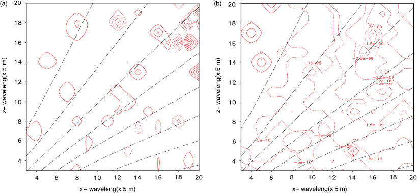
Fig. 2
(a) Frequency of ω δ=16 (Δt=4.71×10⁻² s, dash) from 0.002 (dashed line at right-bottom corner) to 0.009 s−1 with interval of .001 s −1, and ω δ=16−σ g (dot) from –2.5×10⁻⁸ to 2.0×10⁻⁸ s−1 with interval of 1.0×10⁻⁹ s−1; (b) δ=16 (Δt=9.42×10⁻² s and smoothing), and from −3.5×10⁻⁹ to 5.0×10⁻¹⁰ s−1 with interval of 5.0×10⁻¹⁰ s−1.
4. Numerical simulations
The non-linear non-hydrostatic CReSS (Tsuboki and Sakakibara, 2002, 2007), has been applied to simulate shear instability, thermal bubbles, and mountain waves with the FB, MFB, MFBS and HE–VI. CReSS uses Arakawa C and Lorenz staggered grids in the horizontal and vertical, respectively. Prognostic variables consist of the 3-D velocity components, perturbations of pressure and potential temperature, water vapour mixing ratio, subgrid scale turbulent kinetic energy (TKE) and cloud physical variables. In the FB version of CReSS, u, v and w are calculated using forward-differences, while the pressure perturbation p’ uses the backward-difference with a small time interval (Δts). The non-linear and other forcing terms, which are calculated at a larger time interval (Δtb=nΔts), remain constant when integrating sound waves. The leapfrog scheme is applied to the advection terms. The model also includes viscosity and divergence damping of the pressure gradient force in the momentum equations. In the HE–VI, the forward difference is applied to calculate u and v. Then, the implicit scheme is applied to solve w and p’ using a tri-diagonal matrix solver, as discussed in Saito (2007). The detailed equations and numerical schemes are referred to Tsuboki and Sakakibara (2007). There is no analytical solution to the non-linear eqs. (1)–(6). Hence, the results of the conventional FB (δ=1) will be used as the references to compare with the simulations from the HE–VI, MFB and the new MFBS.
4.1. Large Kelvin-Helmholtz wave with Δx =10 m and Δz=5 m
The initial x-component wind u is shown in Fig. 3a. The initial background potential temperature and elliptic-type perturbation with the amplitude of –0.4 K, and the horizontal and vertical radii of 180 m and 60 m are shown in Fig. 3b. Figure 4a shows the simulated potential temperatures θ at t=320 s with Δtb=0.4 s from: FB with Δts=0.01 s; MFB with δ=16, Δts=0.04 s; MFBS with δ=4, Δts=0.04 s; MFBS with δ=16, Δts=0.08 s; and HE–VI with Δts=0.02 s. The five simulations nearly coincide. The differences between θ MFBS(δ=4, Δts=0.04 s) and θ FB (δ=1, Δts=0.01 s) range from –0.03 to 0.03 K, (Fig. 4b). Meanwhile, θ MFBS(δ=16, Δts=0.08 s)–θ FB (δ=1, Δts =0.01 s) is from –0.12 to 0.08 K, (Fig. 4c). Fig. 5b–d of Part I show the differences between the MFB (δ=16, Δts=0.04 s) and FB, which range from –0.12 K to 0.1 K; between the HE–VI (Δts=0.02 s) and FB they are from –0.02 to 0.03 K. The accuracies are comparable between the MFBS with δ=4, Δts=0.04 s and HE–VI with Δts=0.02 s, as well as between the MFB with δ=16, Δts=0.04 s and MFBS with δ=16, Δts =0.08 s. However, the Δts for the MFBS is twice that for the MFB with the same δ. It is also noted that the HE–VI model becomes unstable when Δts=0.04 s.
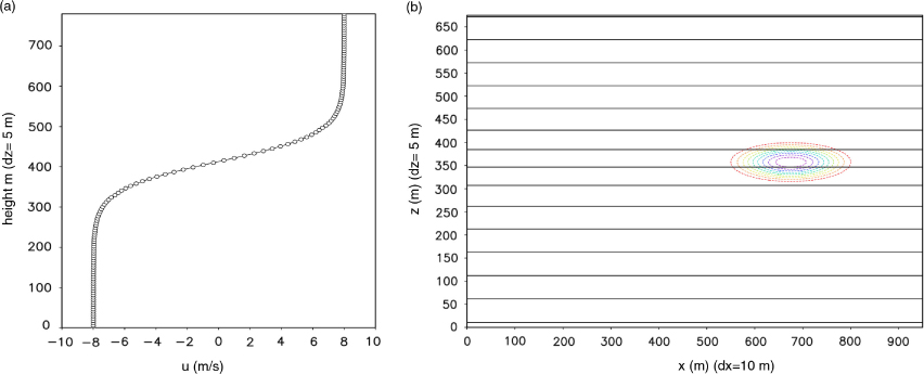
Fig. 3
(a) Initial x-component wind for Kelvin-Helmholtz instability for Section 4.1–4.2; (b) initial background θ 0 (solid) and perturbation θ’ (dot) for large-scale waves discussed in Section 4.1.
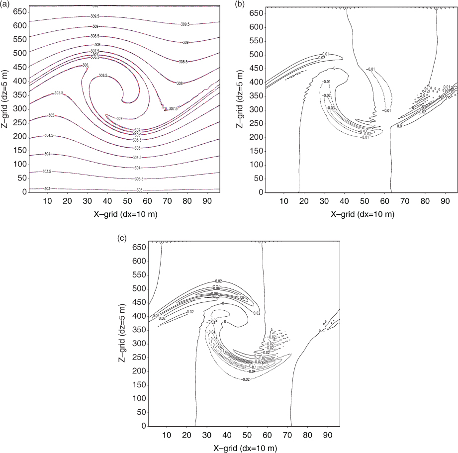
Fig. 4
Simulations for large-scale Kelvin-Helmholtz instability at t=320 s with Δtb=0.4 s from (a) θ FB (δ=1, Δts=0.01 s); MFB (δ=16, Δts=0.04 s); MFBS(δ=4, Δts=0.04 s); MFBS (δ=16, Δts=0.08 s), and HE–VI (Δts=0.02 s); (b) θ MFBS (δ=4, Δts=0.04 s) − θ FB (Δts=0.01 s), contours from –0.03 to 0.03 K with interval of 0.01 K; (c) θ MFBS (δ=16, Δts=0.08 s) −θ FB (Δts=0.01 s), contours from –0.12 to 0.08 K with interval of 0.02 K.
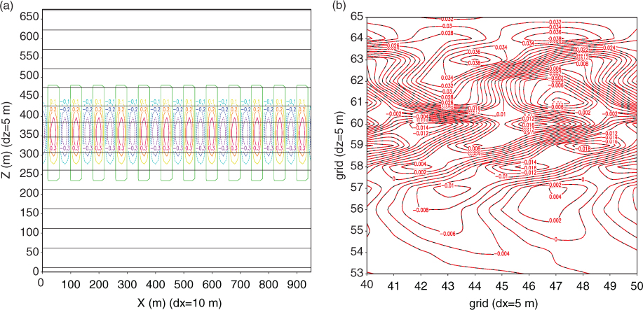
Fig. 5
As above but for small-scale Kelvin-Helmholz instability simulation (a) initial background θ 0 (solid) and perturbation θ’ (dash); (b) simulated θ’ at t=240 s from FB (δ=1, Δts=0.005 s, red solid), and MFBS (δ=16, Δts=0.04 s, blue dash). Contour interval is 0.002 K.
4.2. Small Kelvin-Helmholtz waves with Δx=5 m, Δz=5 m
The initial x-component wind and the background potential temperature are the same as in Section 4.1. The amplitude of initial potential temperature perturbation θ’ is –0.4K, which consists of sine-waves in the horizontal with a wavelength of 40 m and an elliptic-type perturbation in the vertical with a radius of 120 m, as shown in Fig. 5a. Figure 5b shows the simulated θ’ at t =240 s with Δtb=0.12 s from FB with δ=1 and Δts=0.005 s (solid line) and from MFBS with δ=16 and Δts=0.04 s (dashed line). The temperature contours are virtually indistinguishable. The same holds for the velocity fields (not shown). However, the simulated temperature and velocity from HE–VI (Δts=0.005 s) depart significantly from the FB with the same time interval, as discussed in Part I.
4.3. Thermal bubble without mean wind
The initial potential temperature of a thermal bubble with a Gaussian profile is shown in Fig. 8a of Part I, following eqs. (38) and (39) of Robert (1993). Simulations were performed with the same Δx=Δz=5 m and Δtb=0.12 s as in Part I. The simulated θ and velocity vector at t=6, and 12 min of MFBS (δ=16 and Δts=0.06 s) are almost identical to those of FB (δ=1 and Δts=0.008 s) shown in Fig. 8b and c in Part I. Figure 6a shows the simulated θ MFBS (Δts=0.06 s with black contours) and θ FB (Δts=0.008 s with colour shaded plot) at t=18 min for comparison. The difference between θ MFBS and θ FB ranges from –0.03 to 0.04 (Fig. 6b). Between θ MFB (δ= 16, Δts=0.03 s) and θ FB the difference ranges from –0.03 to 0.06 K, and for θ HE–VI (Δts=0.008 s) and θ FB, from –0.3 to 0.2 K, as shown in Fig. 9c and d in Part I. The time interval Δts for the MFBS is twice that for MFB and almost eight times that for HE–VI. Yet, the simulations using MFBS are as accurate as MFB and better than HE–VI. The simulations are also comparable to those of Robert (1993), Hsu and Sun (2001) and Chen and Sun (2001), etc., although the details depend upon the particular numerical schemes and turbulence parameterisations chosen for each model.
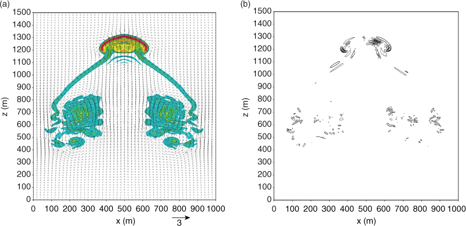
Fig. 6
Simulations at t=18 min: (a) velocity V MFBS and θ MFBS (δ=16, Δts=0.06 s, black contours), and θ FB (Δts=0.008 s, colour shaded), contours from −0.15 to 0.6 K; and (b) θ MFBS (δ=16, Δts=0.06 s) − θ FB (Δts=0.008 s), contours from −0.03 to 0.04 K.
4.4. Thermal bubble with 10 m s−1 mean wind
The initial conditions are identical to those described in Section 4.3, except for the addition of a 10 ms−1 prevailing mean wind. This allows for an interaction between thermal convection and the mean wind, which is a more realistic scenario than the previous case. The simulated potential temperature perturbation and velocity perturbation V’ from the mean wind for the MFBS (δ=16 and Δts=0.06 s) at t=12 and 24 minutes are shown in Fig. 7a and b with a periodic boundary condition. The pattern is almost symmetric at t=12 min and becomes more asymmetric with increasing time, because the x-component wind is slightly stronger on the windward side of the thermal. Figure 7b shows that the warm area shifts to the right-hand side of the front at t=24 minutes. Differences from the FB (Δts=0.008 s) simulations remain small: between –0.004 and 0.006 K at t=12 minutes, and between –0.15 and 0.2 K at t=24 minutes (Fig. 7c and d).
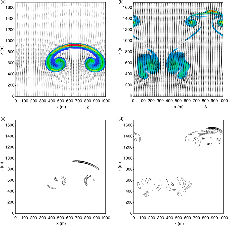
Fig. 7
(a) Simulated velocity perturbation V’ MFBS and θ MFBS (δ=16, Δts=0.06 s) at t=12 min, (b) same as (a) but at t=24 min, (c) θ MFBS−θ FB (Δts=0.008 s) at t=12 min, contours from −0.004 to 0.006 with interval of 0.001, and (d) θ MFBS−θ FB at t=24, contours from −0.015 to 0.02 K with interval of 0.005 K.
4.5. Mountain waves
A uniform 10 m s−1 wind flows over a bell-shaped mountain with a peak height of 500 m and a half-width of 2000 m. The background buoyancy frequency is 0.01 s −1. The simulated w with Δx=400 m, Δz=125 m and Δtb=10 s, at t=9000 s from: FB with δ=1, Δts=0.25 s; MFB with δ=16, Δts=1.0 s; MFBS with smoothing, δ=16, Δts=2.0 s; and HE–VI with Δts=1.0 s are shown in Fig. 8a. They coincide among each other. Figurw 8b shows that the difference in simulated w between the FB (Δts=0.25 s) and MFBS (δ=16, Δts=2.0 s) at t=9000 s ranges from –0.1 to 0.08 m s−1 (solid lines), and the difference between the FB and MFB (δ=16, Δts=1.0 s) is also between –0.1 and 0.08 m s−1 (dashed lines). Similarly, the difference between the FB and HE–VI (Δts=1.0 s) is between –0.1 m s−1 and 0.08 m s−1 (dashed line) in Fig. 8c. Hence, the accuracy is comparable among the MFB (δ=16, Δts=1.0 s), MFBS (δ=16, Δts=2.0 s with smoothing) and HE–VI (Δts=1.0 s).
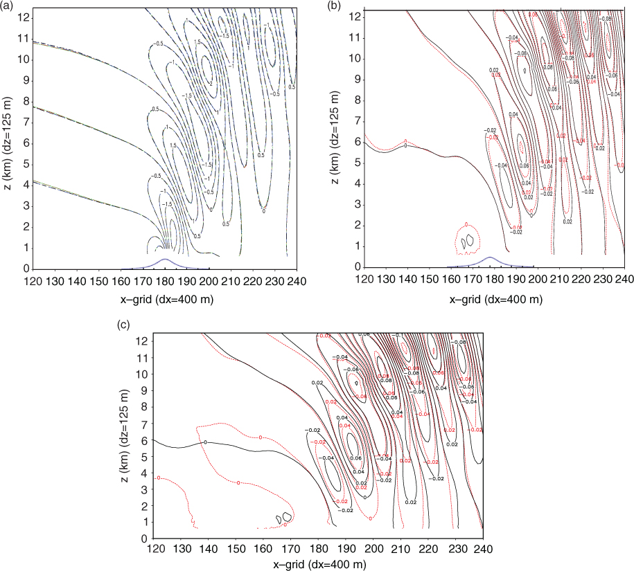
Fig. 8
Simulations at t=9000 s with Δx=400 m, Δz=125 m and Δtb=10 s: (a) w δ=1 (Δts=0.25 s, black dotted); w δ=16 (Δts=1.0 s, red short-dash); w MFBS (Δts=2.0 s, δ=16, green long-dash); and w HE–VI (Δts=1.0 s, blue long-dash, short dash); (b) w δ=16−w δ=1 (red dash) and w MFBS−w δ=1 (black solid); and (c) w HE–VI –w δ=1 (red dash) and w MFBS (δ=16, Δts=2.0 s)–w δ=1 (black solid), the contour interval is 0.02 m s−1.
5. Summary
In Part I, it was demonstrated that the MNH with a parameter δ (between 4 and 16) applied to the continuity equation can suppress high-frequency acoustic waves effectively without a significant impact on gravity waves, enabling the use of a longer time step. Here, we have added a smoothing to the right-hand side of the continuity equation in the MNH, allowing us to double once more the time interval which was used for the MFB in Part I. Both eigenvalue analyses and non-linear model simulations show that the smoothing does not significantly degrade the accuracy of the results. The MNHS approach is simple and can be easily incorporated into many different numerical schemes. Furthermore, the results do not depart from the conventional FB result, even when the time interval used for the MNHS is eight times that for FB. However, HE–VI simulations can be significantly different from FB even when using an identical time interval that is allowed by the CFL criterion, as discussed in Part I. When the aspect ratio is around 6, the same Δts can be applied to the MFBS and HE–VI, but the HE–VI still needs more computing time to solve a tri-diagonal matrix. Besides, the HE–VI results may depart from that of FB, as discussed in Part I. We conclude that the MNHS is more accurate and efficient than the HE–VI when the aspect ratio is small, as in the cases presented here.
Acknowledgements
We would like to thank Profs. Uyeda and Ohigashi, Kato San and Tsujino San at Nagoya University for their help when the senior author was a Visiting Professor at the Hydrospheric Atmospheric Research Center (HyARC), Nagoya University. We also like to thank Mr. Seaman at Purdue Information Technology Center for his assistance during this study. The reviewers’ comments are greatly appreciated. The computing facilities provided by Nagoya University, Purdue University and Taiwan High Performance Computing Center are highly appreciated as well.