Fig. 1.
The zonal average, monthly average zonal wind (red contours, labelled in m s−1), potential vorticity [green contours, labelled in PVU; interval is 50 PVU (1 PVU=1 K m2 kg−1 s−1) for absolute values greater than 50] and pressure (black dashed contours, labelled in hPa) as a function of potential temperature and latitude according to the CIRA (Appendix) for January and July. The monthly average overhead position of the sun is indicated in red below each figure.
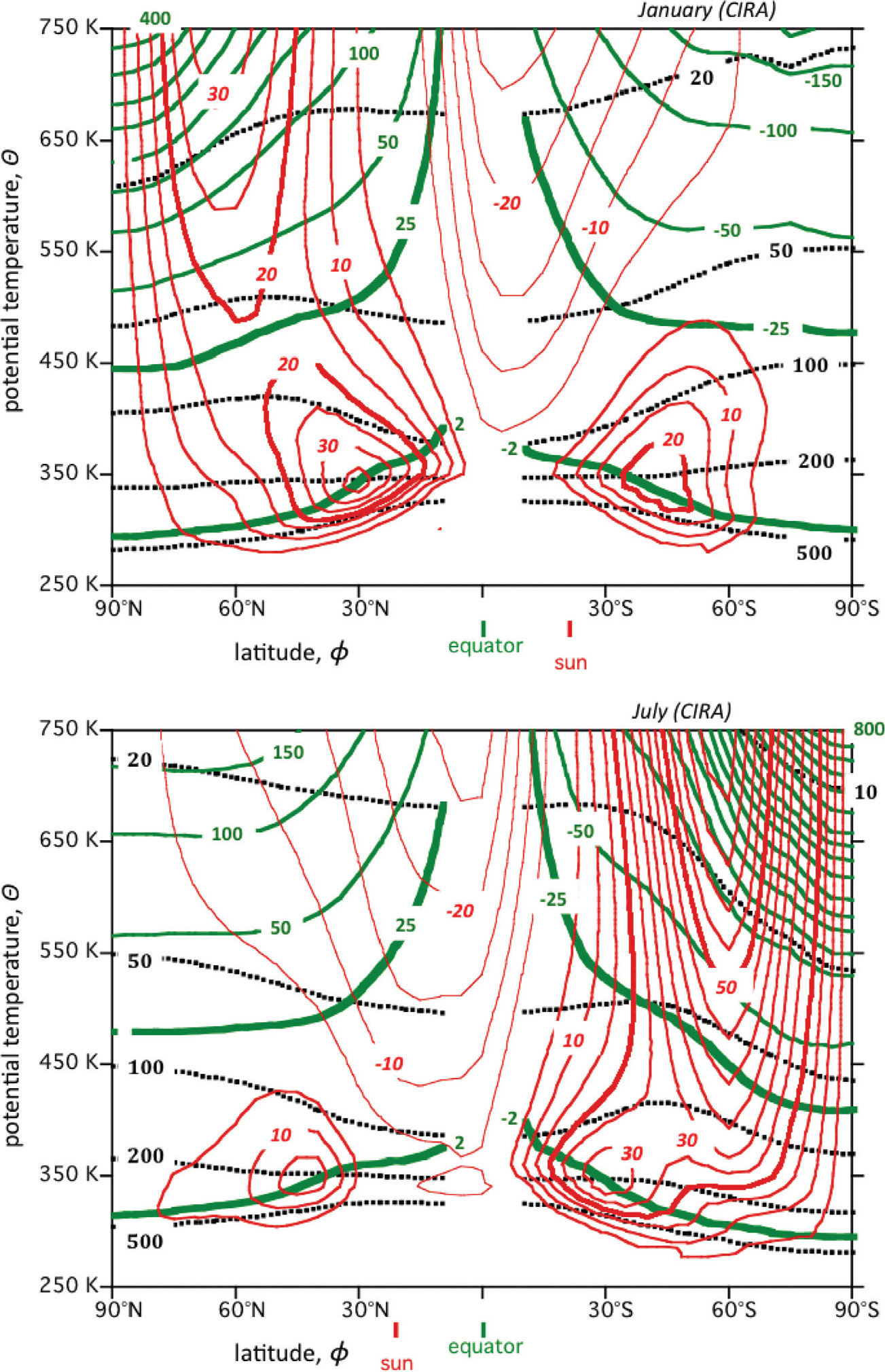
Fig. 2.
The average reference isentropic density, where the integral in eq. (14) is taken from 10°N to the North Pole, for January (blue solid line) and for July (red solid line), and the zonal average isentropic density at 60°N (January average: blue dashed line; July average: red dashed line) as a function of potential temperature, based on the CIRA (Appendix).
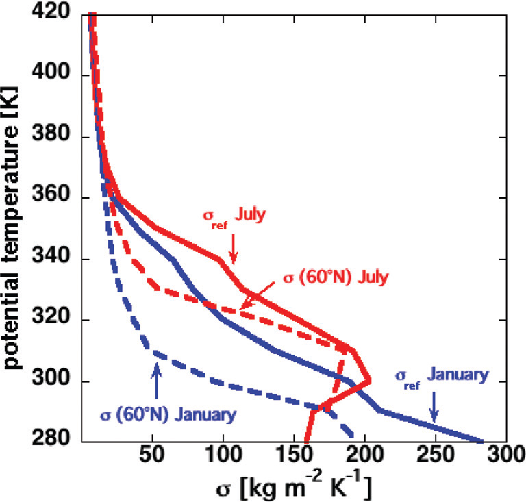
Fig. 3.
The zonal average distributions of Z ref (green contours; labelled in PVU), Z* (red: positive; blue: negative; labelled in non-dimensional units) and pressure (dotted; labelled in hPa) as a function of latitude and potential temperature for January and July. Plus and minus signs indicate maxima and minima in Z*, respectively. Contours within 10° of the equator are not drawn, based on the CIRA (Appendix). The thick black line corresponds to the Earth's surface (see caption of Fig. 1 for more information). The contours of Z* correspond to the values, ±0.1, ±0.5, ±1, ±2 and ±3 units.
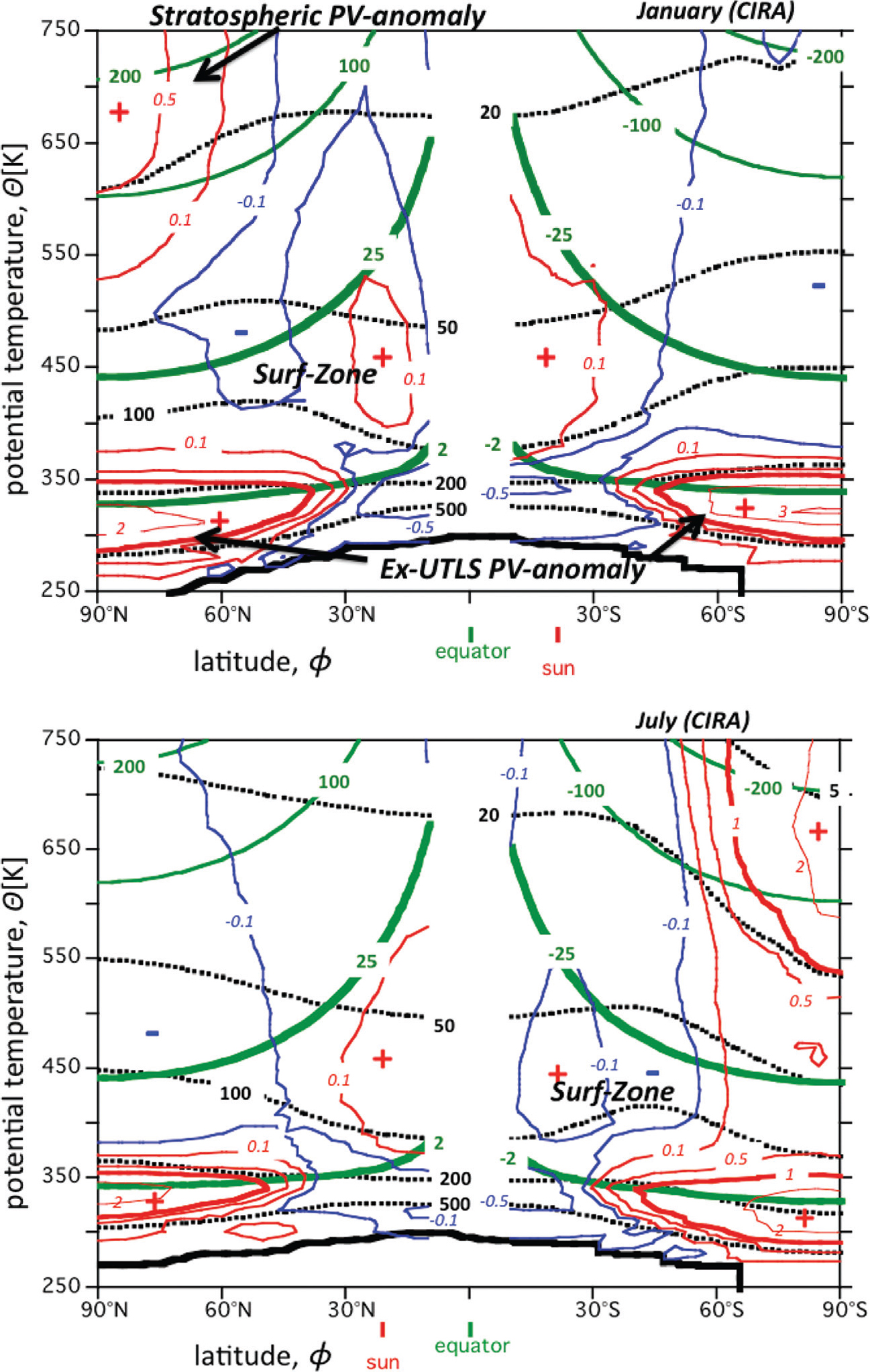
Fig. 4.
The monthly mean, zonal mean normalised relative vorticity anomaly, б* in January and in July, labelled in non-dimensional units (red: positive; blue: negative), based on the CIRA (Appendix). Also shown is pressure (dashed lines, labelled in hPa). The positive stratospheric polar cap PV-anomaly in the winter hemisphere is manifest more strongly as a vorticity anomaly than the Ex-UTLS PV-anomaly.
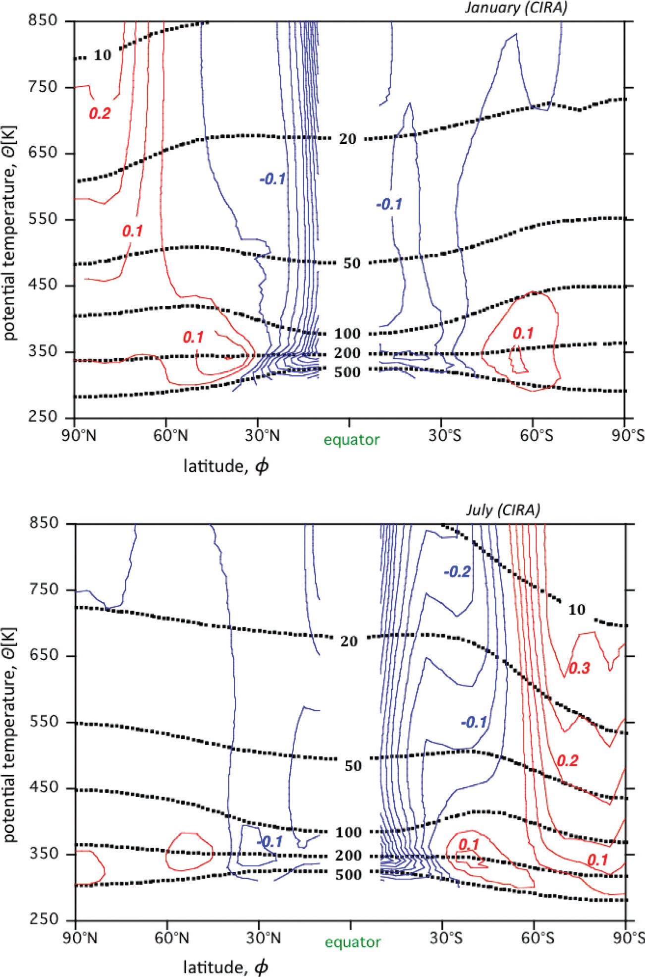
Fig. 5.
The monthly mean, zonal mean normalised isentropic density anomaly, σ*, in January and in July, labelled in non-dimensional units (blue: positive; red: negative), based on the CIRA (Appendix). Also shown is pressure (dashed lines, labelled in hPa). The positive Ex-UTLS PV-anomaly manifest very strongly as a negative mass anomaly. The stratospheric polar cap PV-anomaly in the winter hemisphere is manifest more strongly as a negative mass anomaly in the Southern Hemisphere than in the Northern Hemisphere.
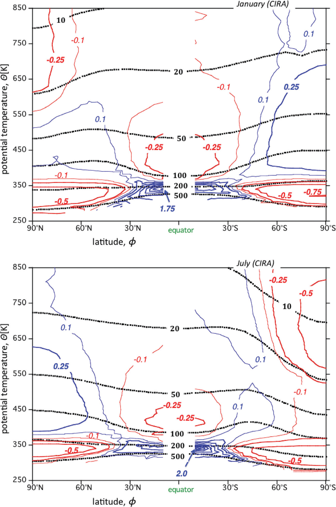
Fig. 6.
The approximate position of the Earth's surface (according to the CIRA, this coincides with p=1013 hPa), relative to the numerical grid in the Northern Hemisphere in January, is indicated by the blue line and open squares. The red line indicates the potential temperature of the lowest computational level for January. The black solid squares indicate the grid points that are located at the southern side-boundary of the computational grid. Thermal wind balance is applied to the lowest computational layer (indicated by double arrows) using the CIRA analysis of the isobaric potential temperature gradient at 1013 hPa [eq. (21)].
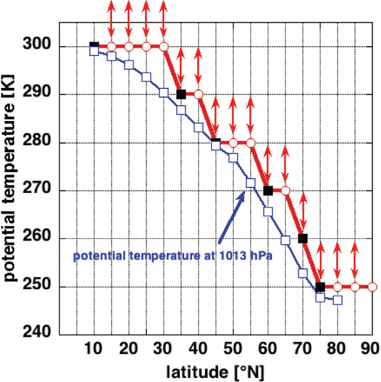
Fig. 7.
Thermal wind Δu in January (blue solid line) and July (red solid line) as a function of latitude in the lowest computational layer (Fig. 6), derived from the monthly average zonal average temperature and pressure analysis according to the CIRA, using eq. (21) with f loc=f. Also shown is the wind shear (m s−1) across the lowest computational layer according to the CIRA (red circles: July; blue squares: January).
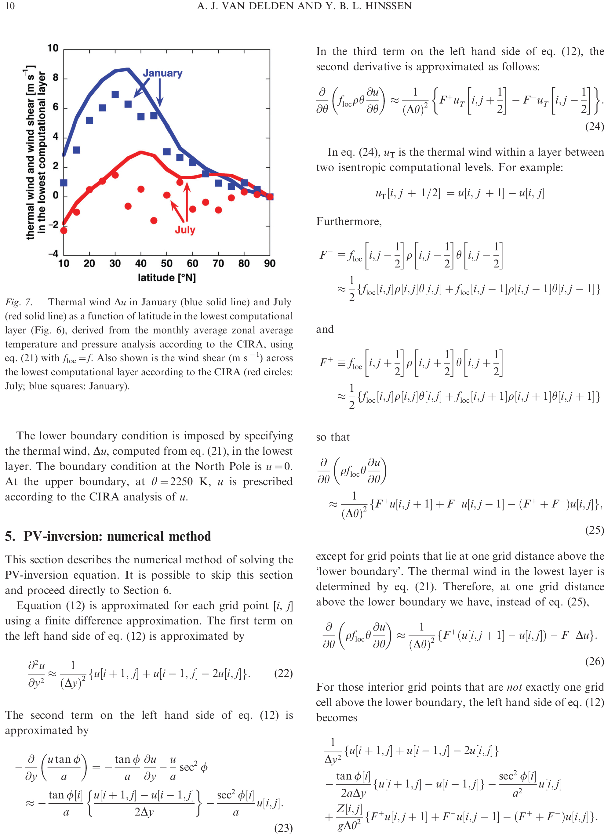
Fig. 8.
The zonal average, monthly average zonal wind velocity as a function of potential temperature and latitude (black contours, labelled in m s−1) in January, derived from PV-inversion (left panel) and according to the CIRA (right panel). The normalised PV-anomalies that ‘induce’ this wind field are shown in blue (only positive values are contoured). Labels are given in non-dimensional units. The isopleths corresponding to 0.1 and 1 non-dimensional unit are drawn thick; the isopleths corresponding to 0.5, 2 and 3 non-dimensional units are drawn thin. For more details of the structure of these anomalies, see Fig. 3.
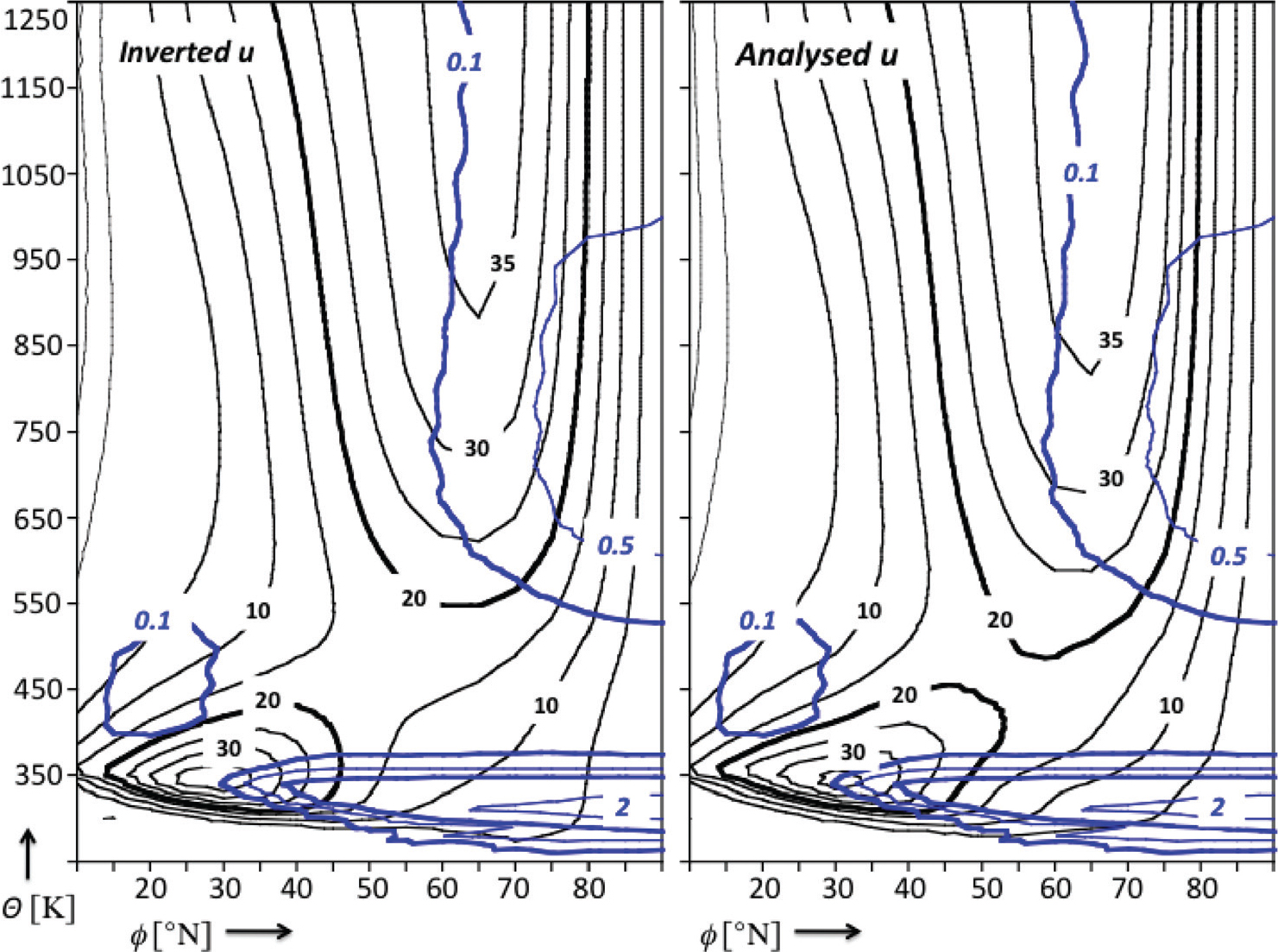
Fig. 9.
Left panel: the difference between the analysed wind and the inverted wind for January (labelled in units of m s−1). Right panel: the difference between the sum of the two piecewise inverted wind fields (shown in Fig. 10) and the wind field obtained from inversion of the total PV-field, shown in the left panel of Fig. 8. Labels are in units of m s−1. The inverted pressure field is also shown (dashed lines labelled in units of hPa).
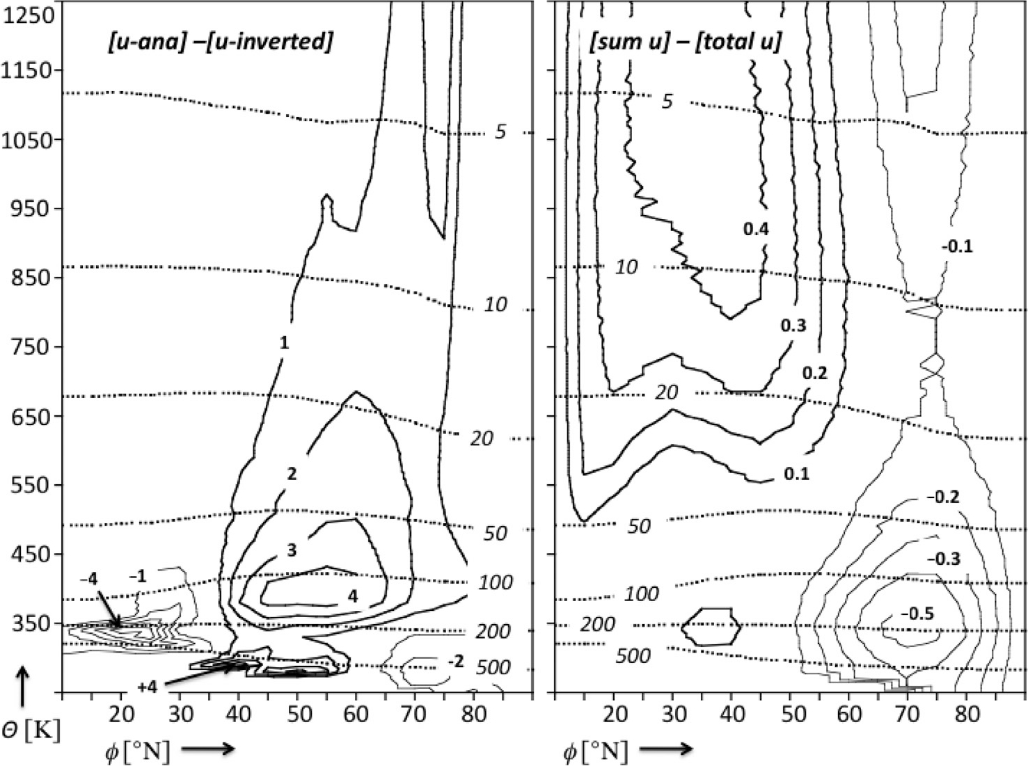
Fig. 10.
The zonal average, January average zonal wind velocity (black contours, labelled in m s−1) and pressure (dashed lines, labelled in hPa) as a function of potential temperature and latitude, derived from piecewise PV-inversion. Left panel shows the result when the Ex-UTLS PV-anomaly and the surface temperature anomaly are retained (i.e. Z*=0 for θ=480 K). The right panel shows the result when only the polar cap upper stratospheric PV-anomaly is retained (i.e. Z*=0 for θ≤480 K and Δu=0) and the zonal wind according to the CIRA is imposed at the top boundary at 2250 K. The PV-anomalies that are retained in the inversion are shown in blue and labelled in non-dimensional units as in Fig. 8 (only positive values are contoured).
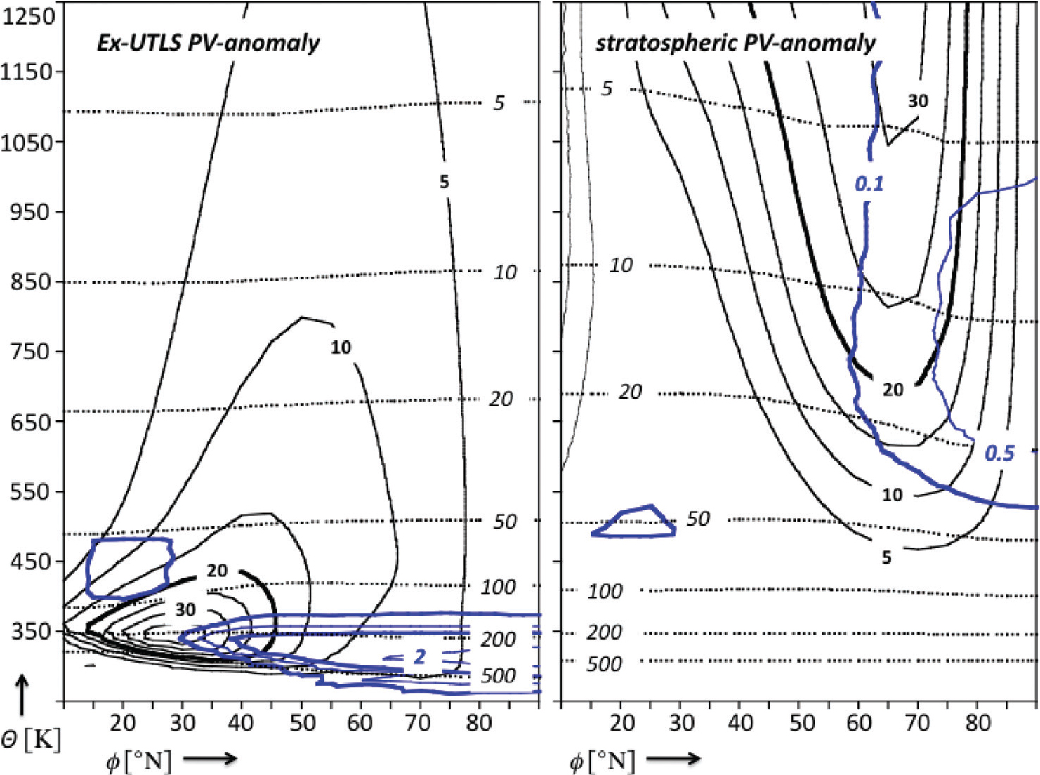
Fig. 11.
The zonal average, monthly average zonal wind velocity as a function of potential temperature and latitude (black contours, labelled in m s−1) in July derived from PV-inversion (left panel) and according to the CIRA (right panel). The normalised PV-anomalies that ‘induce’ this wind field are shown in colours (negative values in red; positive values in blue; labelled in non-dimensional units as in Fig. 8). Also shown is pressure (dashed lines, labelled in hPa).
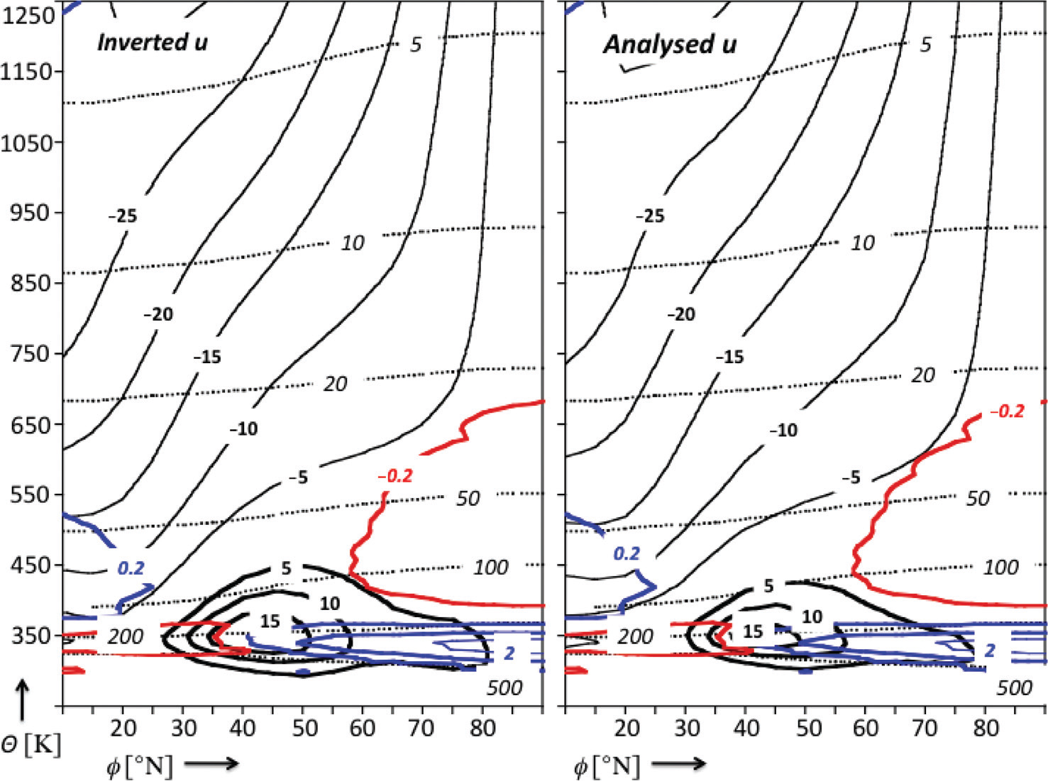
Fig. 12.
The zonal average pressure anomaly at 300 K in July in the Northern Hemisphere, which results after removing the PV-anomaly above 370 K and redistributing the associated mass anomaly, i.e. effectively transferring mass from the extra-tropics to the tropics. The boundary condition must be corrected for this effect.
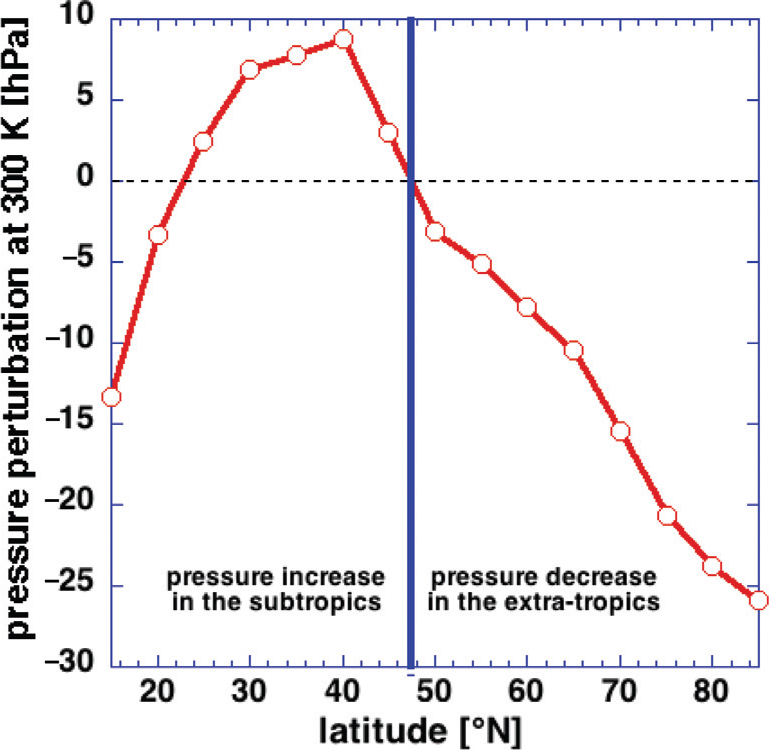
Fig. 13.
The zonal average, July average zonal wind velocity as a function of potential temperature and latitude (black contours, labelled in m s−1) according to the solution of the PV-inversion when Z*=0 for θ>370 K (only positive values of Z*, labelled in non-dimensional units as in Fig. 8, are shown in blue). Left panel: case where the thermal wind at the lower boundary is not corrected; right panel: case where the thermal wind at the lower boundary is corrected for the redistribution of mass.
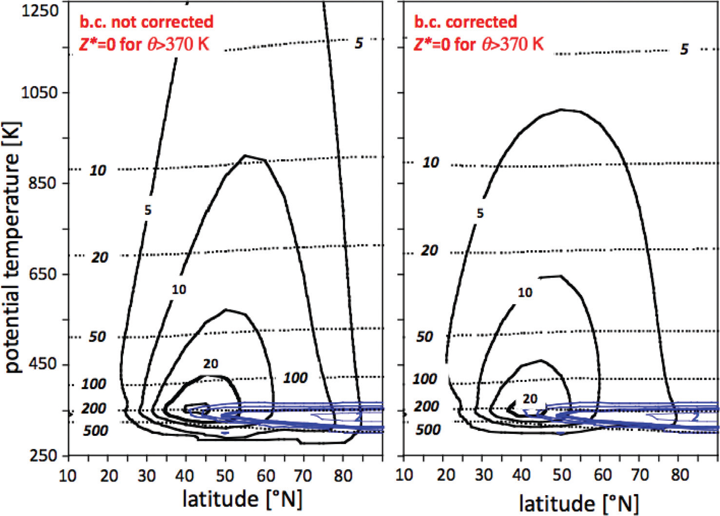
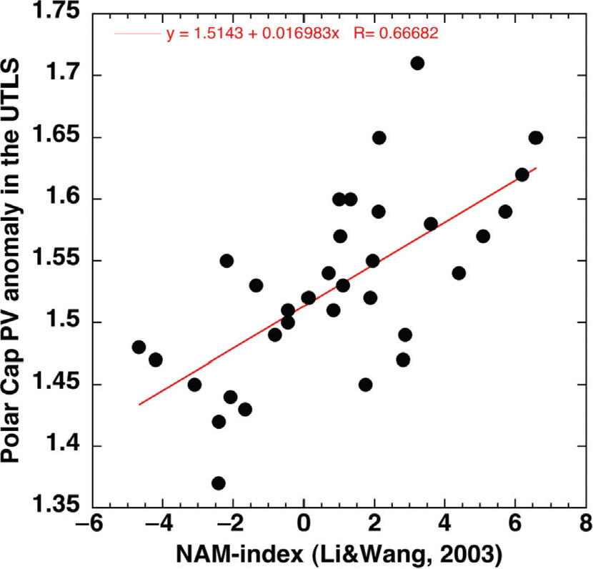
Fig. 14.
Scatter plot of the monthly mean (January of the years 1979–2011) polar cap normalised potential vorticity anomaly, Z*, averaged over the layer between 300 and 370 K, north of 65°N, and the monthly mean Northern Annular Mode (NAM) Index, which is defined as the difference in the normalised monthly zonal-mean sea level pressure between 35°N and 65°N (Li and Wang, 2003). The red line represents the best linear fit to the 33 points with a correlation coefficient of 0.67. The monthly mean potential vorticity is derived from the ERA-Interim reanalysis (Dee et al., 2011).