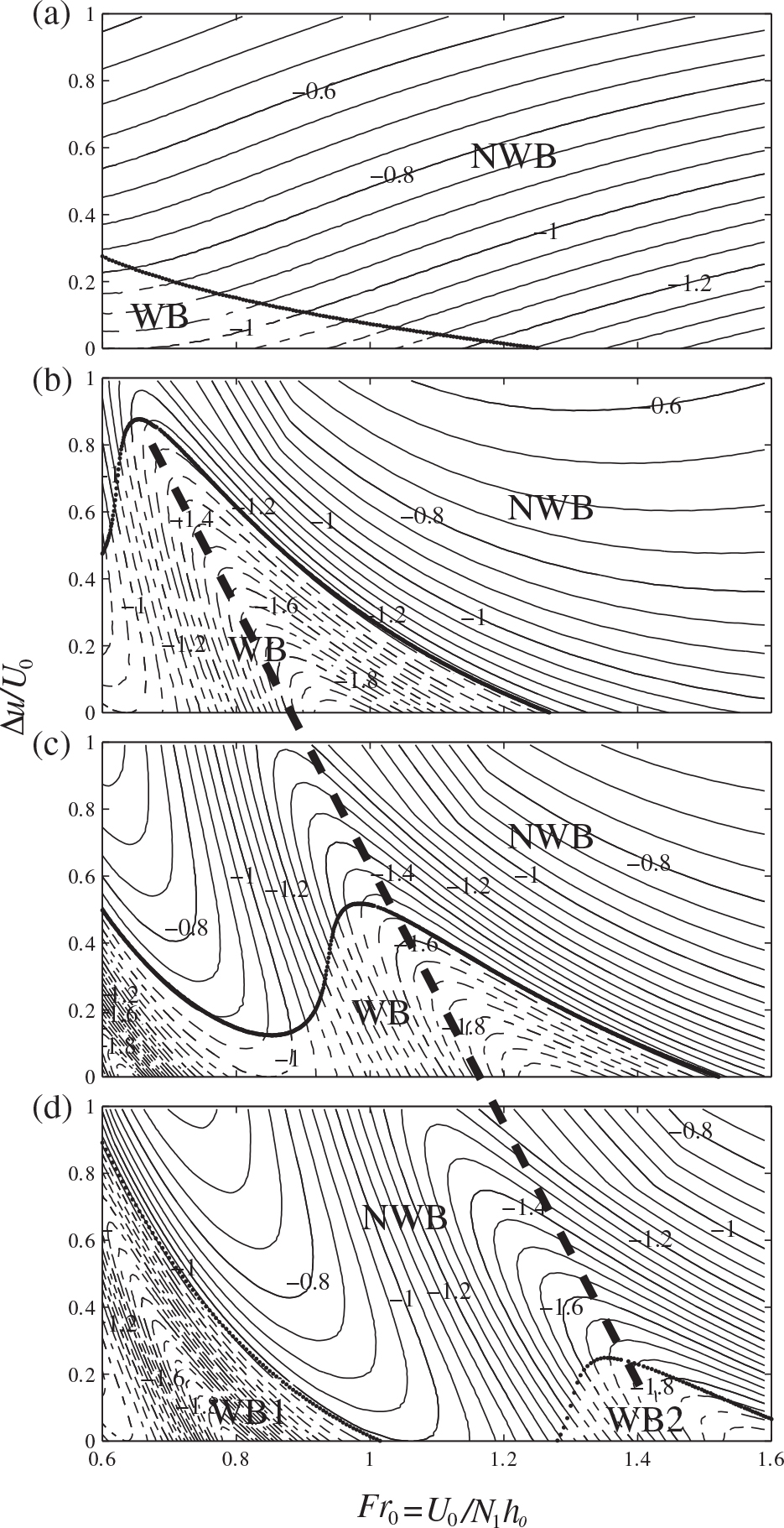
Fig. 1.
Vertical profiles of Brunt–Väisälä frequency and basic wind speed. U 0 is surface wind speed, and Δu is the low-level VWS.
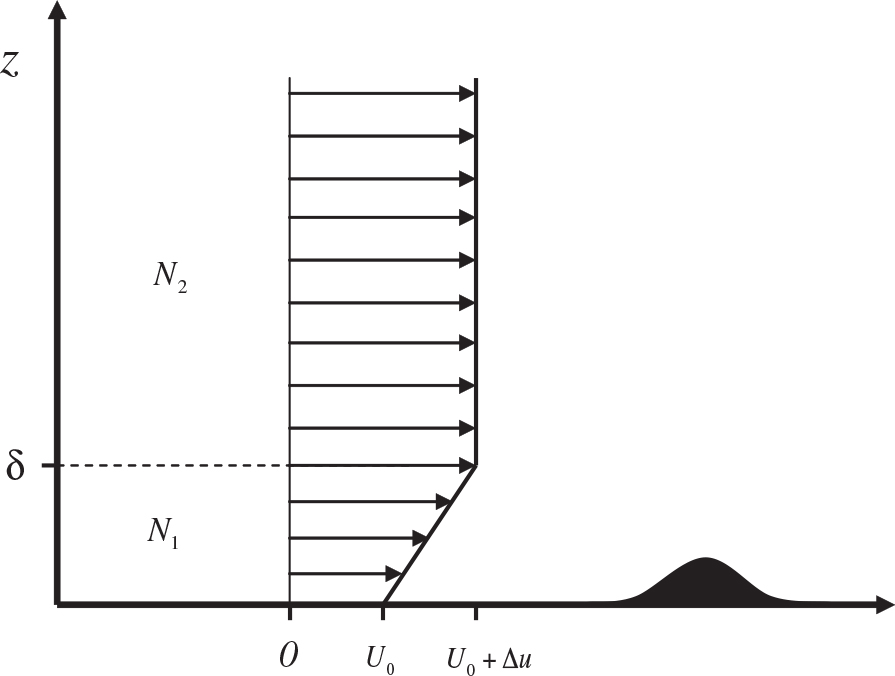
Table 1. Experimental designs and results
Fig. 2.
Surface wind speed and its one-to-one correspondence to low-level VWS when the stagnation point starts appearing over the leeside in Exps CTRL (B1), B2, and B3. Dots, triangles, and asterisks denote Exps CTRL, B2, and B3, respectively.
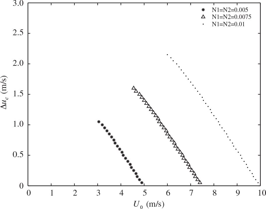
Fig. 3.
Normalised MNHWP (u/N 1 h) for different non-dimensional values of Fr 0 and Δu/U 0. The dotted line denotes the points for Fr 0 and the corresponding Δu c/U 0when the stagnation just appears over the leeside. ‘NWB’ denotes the region with no wave breaking (solid contour); ‘WB’ denotes the region with wave breaking (dashed contour). (a) Exp A1; (b) Exp CTRL; (c) Exp C1; and (d) Exp D1.
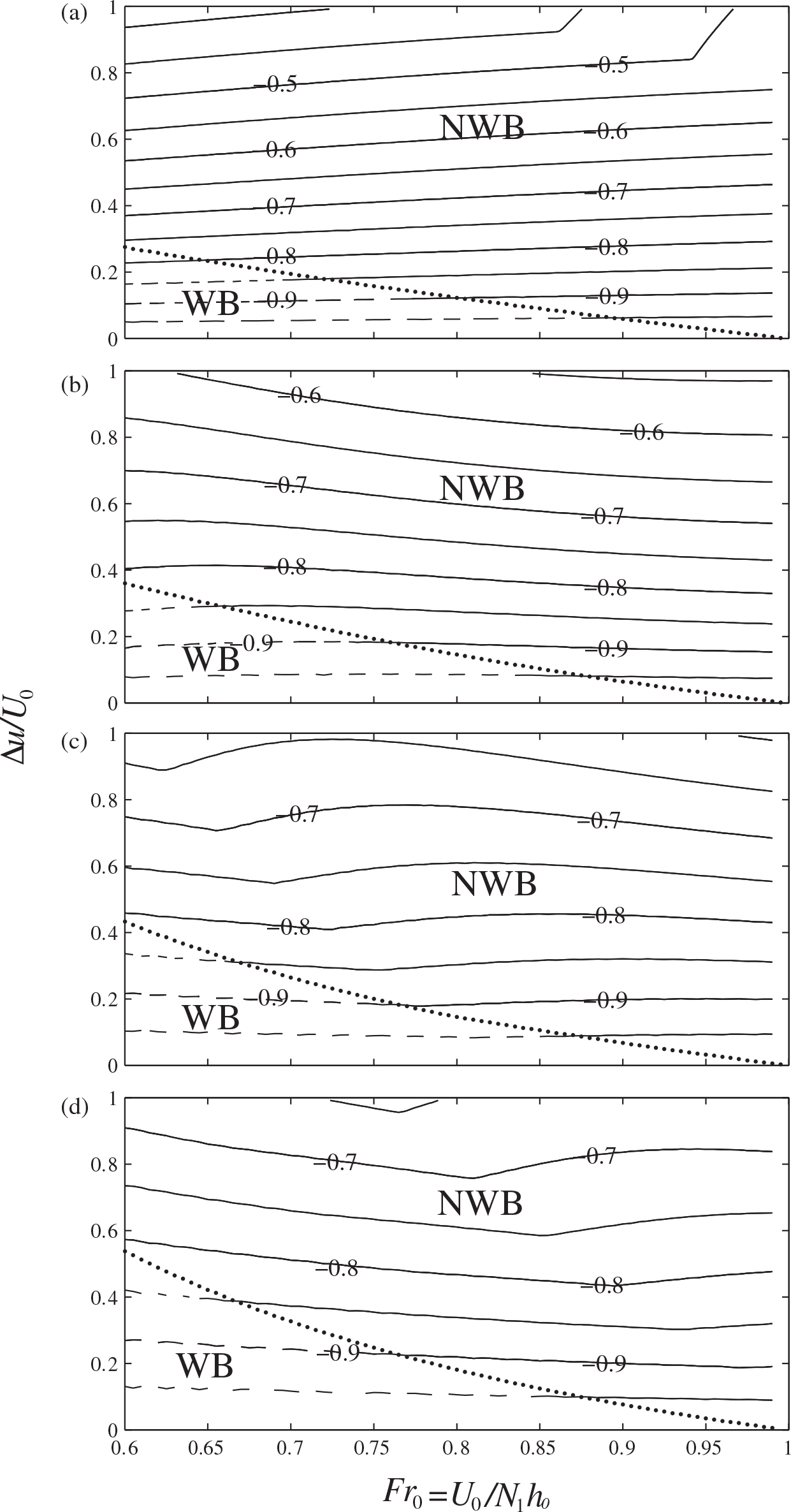
Fig. 4.
Horizontal perturbation velocity (contour interval of 2 ms−1) in CTRL with Δ=3 km and N 1=N 2=0.01 s−1. (a) U 0=10 ms−1, Δu=10−4 ms−1; (b) U 0=15 ms−1, Δu=10−4 ms−1; and (c) U 0=10 ms−1, Δu=5.0 ms−1.
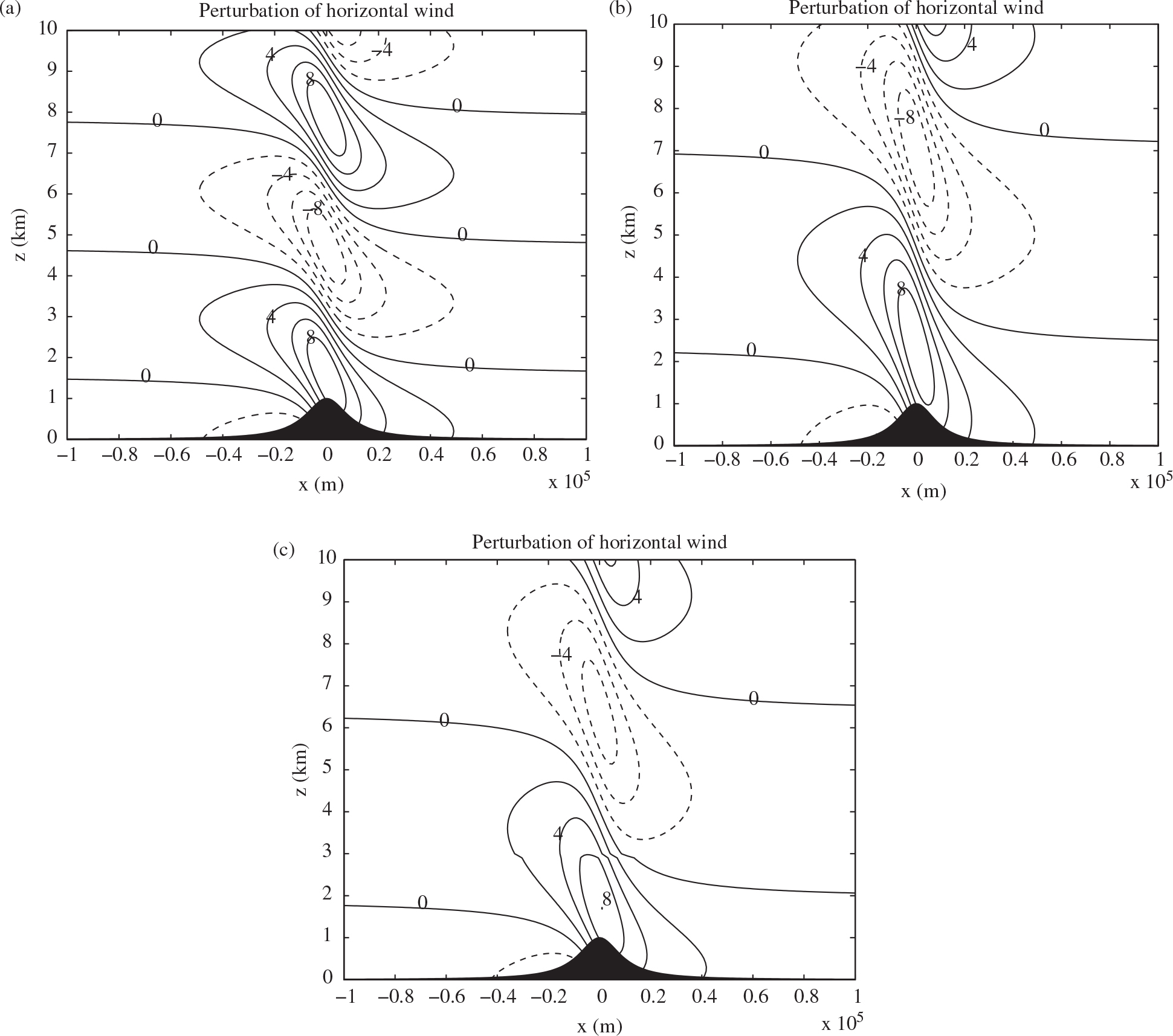
Fig. 5.
Vertical configuration of the Brunt–Väisälä frequency (N 2/N 1) and corresponding Δu max/U 0m for different shear layer depth (Δ). Asterisks, hollow circles, crosses, and triangles denote Δ=1, 3, 4 and 5 km, respectively.
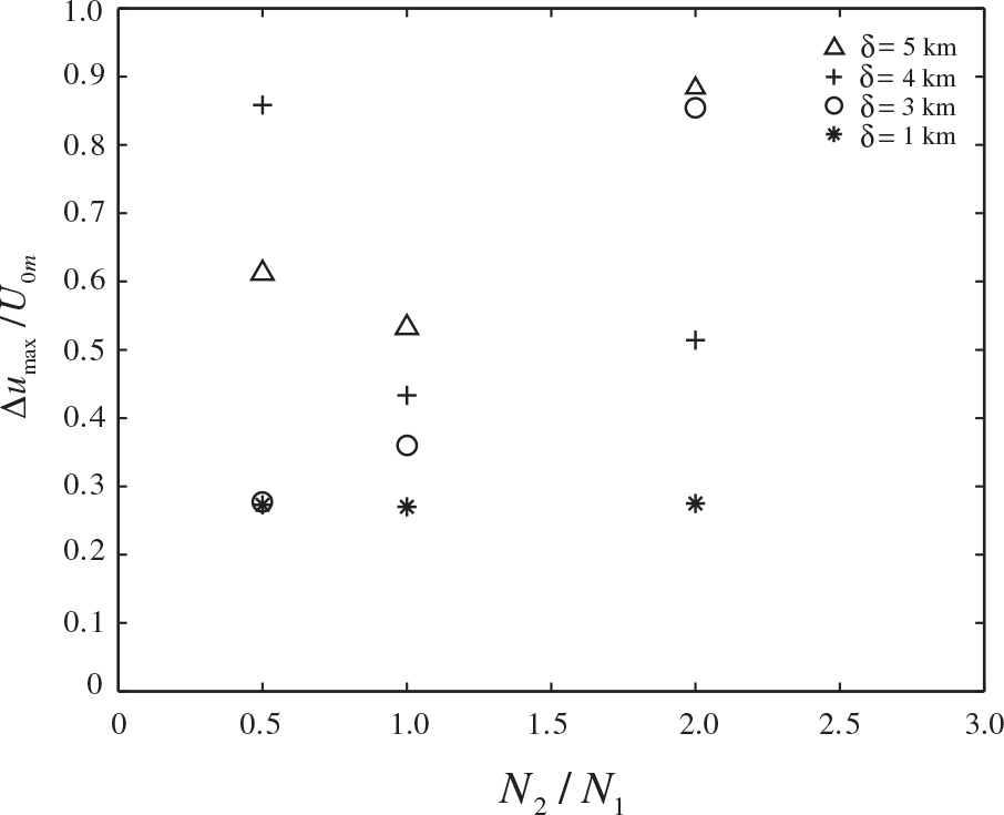
Fig. 6.
Vertical position of stagnation point (black point) calculated using the parameter-space search method. (a) Case 1 with N 2/N 1=1.0; (b) Case 2 with N 2/N 1=0.5; and (c) Case 3 with N 2/N 1=2.0.
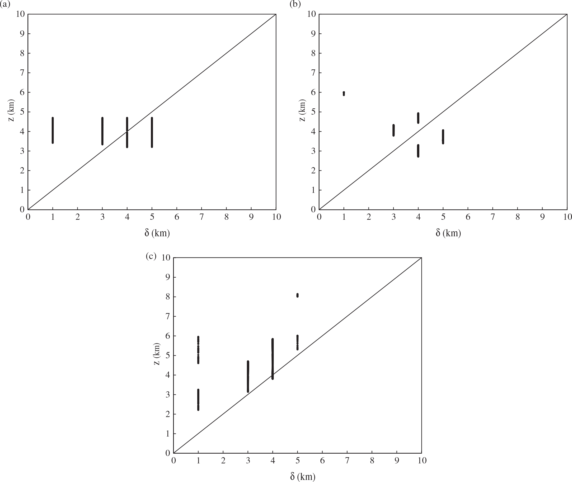
Fig. 7.
Same as in Fig. 4, but for: (a) U 0=10 ms−1, Δu=10−4 ms−1 in Exp D1; (b) U 0=10 ms−1, Δu=10−4 ms−1 in Exp D4; (c) U 0=10 ms−1, Δu=10−4 ms−1 in Exp D5; (d) U 0=16 ms−1, Δu=10−4 ms−1 in Exp D5.
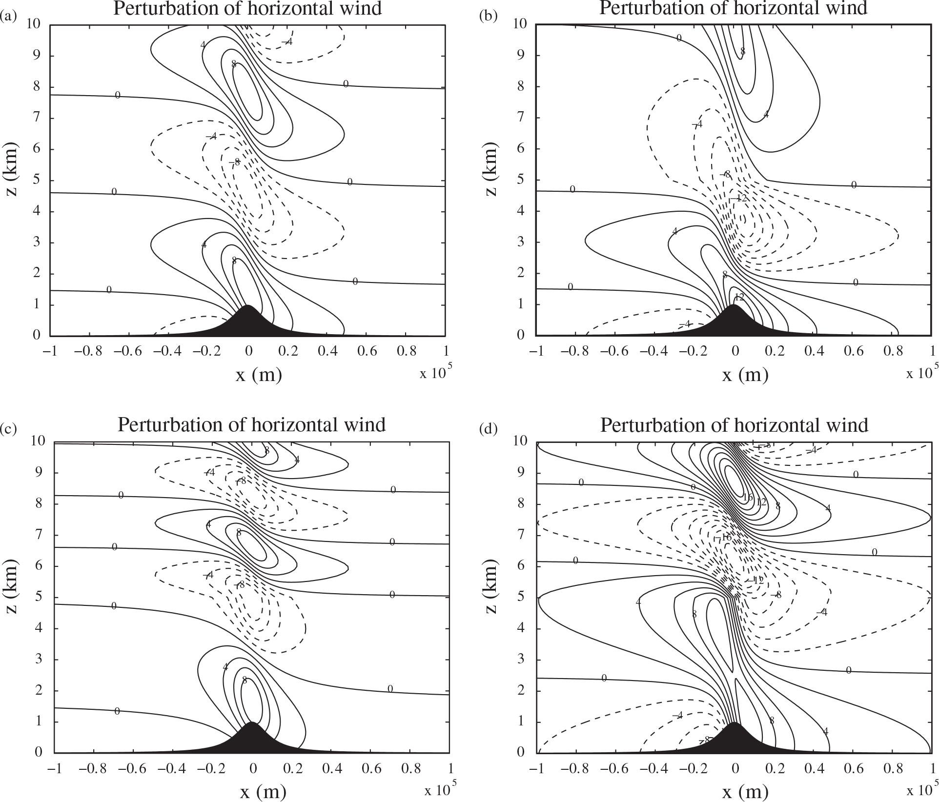
Fig. 8.
As in Fig. 3, but: (a) Exp A4; (b) Exp B4; (c) Exp C4; and (d) Exp D4.
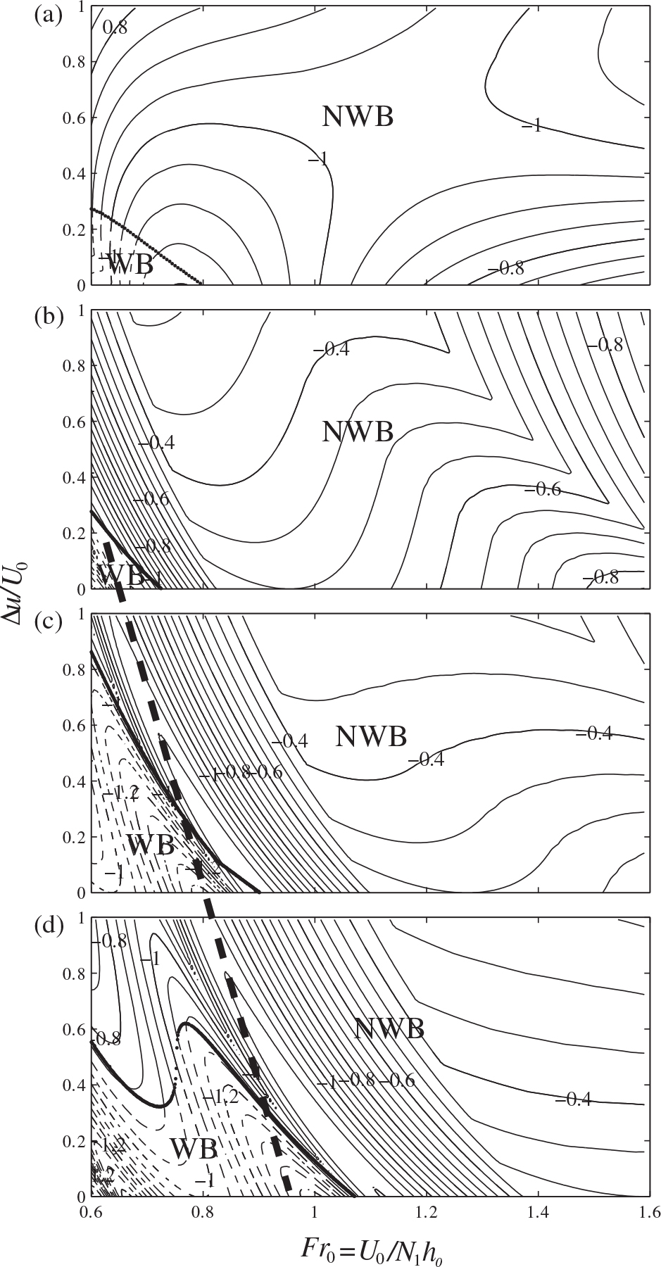
Fig. 9.
As in Fig. 3, but: (a) Exp A5; (b) Exp B5; (c) Exp C5; and (d) Exp D5.