
1. Introduction
Effects of topography on weather and climate have been widely studied for several decades. When an incoming flow imposes on an isolated orography, different regimes of orographic flow may appear, such as flow blocking, gravity wave breaking (GWB), downslope windstorm, downstream waking and trapped wave on the leeside (Smith, 1979). These flow regimes have been extensively investigated using observations, theoretical analyses and numerical simulations.
The classification of orographic flow regimes is closely related to two stagnation points. One is related to the blocking, which occurs at the lower boundary of the windward slope, and another is attributed to the formation of GWB over the leeside. Smith (1989), Baines and Smith (1993) extended Sheppard's theory (Sheppard, 1956) to investigate the influences of atmospheric stratification on the flow regimes and concluded: (i) the amplitude of orographic disturbances is height-dependent; and (ii) the shape of orography can influence the orographic flow. In order to understand the flow regimes, two non-dimensional parameters were introduced: U/Nh and Na/U, where U, N, h, and a are upstream horizontal wind velocity, Brunt–Väisälä frequency, mountain height and mountain half-width (Miles and Huppert, 1969). U/Nh is the Froude number (Fr=U/Nh) that measures the degree of linearity, and Na/U measures the degree of hydrostaticity. Using the two parameters, Rotunno and Ferretti (2001) presented a systematic classification on the flow regimes for a two-dimensional (2-D) flow over an isolated orography (see their Fig. 11). Lin and Wang (1996) synthesised previous studies (e.g. Miles and Huppert, 1969; Baines and Hoinka, 1985; Pierrehumbert and Wyman, 1985; Smith, 1985), and proposed four regimes for the 2-D, non-rotating, uniform Boussinesq, continuously stratified hydrostatic flow over an isolated bell-shape hill based on idealised non-linear numerical simulations: (1) regime I: flow with both wave breaking and upstream blocking, but upstream blocking occurs first (0.3 ≤ Fr<0.6); (2) regime II: flow similar with regime I, but the wave breaking occurs first (0.6 ≤ Fr≤0.9); (3) regime III: flow with only wave breaking aloft (0.9 < Fr≤1.12); and (4) regime IV: flow with neither wave breaking aloft nor upstream blocking (Fr>1.12. Obviously, these four flow regimes are mainly associated with two flow characters, namely, flow blocking and GWB.
GWB is characterised by strong turbulent mixing with flow stagnation or local wind reversal over mountain, and the streamline on the top of orography becomes more steep and vertical. Base on the hydrostatic solution of Long's model for a bell-shaped mountain, Miles and Huppert (1969) identified the non-dimensional mountain height (H=hN/U=0.85) that separates orographic flows into supercritical and subcritical regimes, or wave breaking and no wave breaking. On the other hand, Laprise and Peltier (1989) proposed a critical value of hN/U=0.78 for a semi-circle obstacle, suggesting that the orographic shape is an important factor for GWB's occurring.
To simplify the problem, aforementioned studies for understanding orographic flows often adopted an assumption that the upstream incoming flow is uniform. However, in the real atmosphere there always exists a low-level vertical wind shear (VWS) (Poulos et al., 2002; Woods and Smith, 2011), which is an important factor for the development and maintenance of convective storm (Thorpe et al., 1982). Moreover, VWS can also influence the overturning on the upslope and downslope subsidence over the leeside of the terrain. Concretely, Smith (1989) suggested that VWS can bring on two effects: reducing the effective stability of the orographic flow and making the value of effective non-dimensional mountain height (H=hN/U) rise rapidly for GWB. He even speculated that when the VWS (or the Richardson number) exceeds some value (Ri<20), there will be no GWB occurring aloft, as is a ubiquitous atmospheric condition in the mid-latitude. However, how VWS influences orographic flows and GWB's occurring has not been widely studied so far.
The objective of this study is to investigate the effects of VWS on the GWB's occurring over an isolated orography. In particular, we seek to explore the following three questions. (1) Why can VWS suppress the GWB's occurring (2) Is there a maximum VWS (MVWS) for GWB's occurring, or not? And if the answer is yes, once the VWS is larger than the MVWS, will there be GWB's occurring (3) What are the controlling factors for the MVWS?
Since the lacking of specified observation and 2-D or 3-D simulation on the VWS's impact to GWB, and the complexity of such problem, a 2-D simplified theoretical orographic flow model is used in the present study. Similar to the previous theoretical study on the orographic flow, the simplified model could include the leading-order effect of VWS on the mountain wave. Also the possible errors of such model are discussed.
This paper is organised as follows. A two-layer linear model with the hydrostatic stratified flow over a 2-D, bell-shape orography is briefly described, and the analytical solutions of this model are presented in Section 2. The influence of VWS on orographic flows and the conditions of GWB's occurring are discussed in Section 3. Concluding remarks are given in Section 4.
2. Two-layer linear model and its solution: low-level wind shear case
Similar to Wang and Lin (1999), the linear governing equations for a 2-D, steady-state, non-rotating and hydrostatic flow over orography are given as follows:




where u and w are the perturbations of horizontal and vertical velocities, respectively; U denotes the basic horizontal wind that varies with height, U=U(z); φ is perturbation geopotential height (φ=gz); and b is the buoyancy perturbation, .
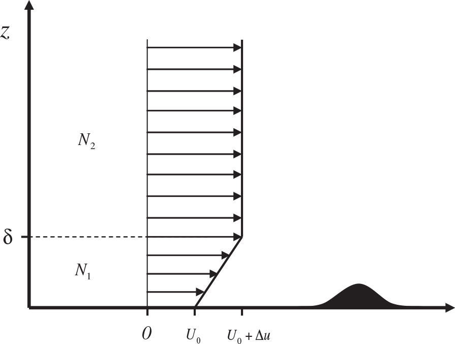
The 2-D flow over orography is assumed to have two layers in the vertical. In the lower wind shear layer (0 ≤ z<Δ), where Δ is the thickness of VWS layer, the horizontal basic flow is westerly and its speed increases linearly with height from U 0 at the surface up to (U 0+Δu) at the height of Δ, where Δu is the VWS. The Brunt–Väisälä frequency of N 1 is a constant in this layer. The upper layer is a uniform wind layer (z≥Δ), where the horizontal basic wind speed and Brunt–Väisälä frequency are both constants, namely, (U 0+Δu), and N 2 (Fig. 1).
Fig. 1.
Vertical profiles of Brunt–Väisälä frequency and basic wind speed. U 0 is surface wind speed, and Δu is the low-level VWS.
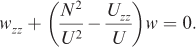
Using eqs. (1)–(4), the equation for the vertical velocity can be obtained:
Similar to Wang and Lin (1999), a one-sided Fourier transform pair is adopted:


Substituting eq. (7) into eq. (5), the Scorer's Equation (Scorer, 1949) is obtained:
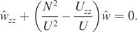
Consequently, the governing equation of in each layer becomes:


At the interface between the two layers, in order to keep the continuity of perturbation pressure and vertical velocity field, we have:

The profile of the bell shape orography is given by:
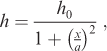
where h 0 is the orographic height, and a is the orographic half-width. In the present study, it is assumed that the height of shear layer is no smaller than the height of orography, i.e. Δ≥h 0. Therefore, the lower boundary condition is given as follows,

After taking the Fourier transform, eq. (13) becomes

With eq. (14), the solutions of eqs. (9) and (10) can be obtained:
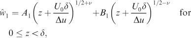

where for Ri < 1/4, and for Ri≥1/4. is the Richardson number. The solutions have the form of lee-wave solution analysed by Wurtele (1957) and Wurtele et al. (1987).
Assume the mountain wave propagates upward, the upper radiation condition is open, so B 2 =0 (Booker and Bretherton, 1967). The other coefficients are:



where:
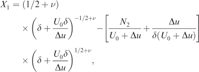
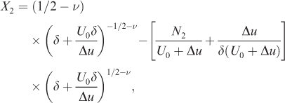
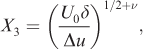
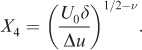
Finally, applied with the inverse Fourier transform, the perturbations of horizontal and vertical velocities in the physical space can be obtained:
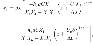

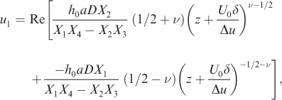

where:
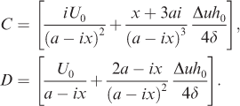
u 1 and w 1 are the perturbations of horizontal and vertical velocities in the lower wind shear layer, respectively; u 2 and w 2 denote those in the upper uniform layer.
3. Conditions for GWB occurring under VWS
In order to investigate the effects of VWS on GWB, the flow regime associated with the upstream blocking is excluded; that means the upstream blocking is assumed to have no impact on the formation of GWB. However, in the real atmosphere many factors can influence the upstream blocking or GWB, which is rather difficult to analyse (Baines and Hoinka, 1985; Pierrehumert and Wyman, 1985; Smith and Gronas, 1993). In order to simplify problem, the surface Froude number (Fr 0=U 0/N 1 h 0) is used to be as a control parameter for the occurring of flow blocking and GWB, which is similar to what used in most studies of 2-D orographic flow. Moreover, based on the previous theoretical and numerical studies on 2-D orographic flow, a reference range of surface Froude number Fr 0 is selected, so Fr b≤Fr 0≤Fr d, where Fr b and Fr d are the critical lower and upper surface Froude numbers. Thus, there is only GWB's occurring, or the GBW's occurring is earlier than the formation of upstream blocking when Fr 0 is larger than Fr b while Fr 0 must be smaller than Fr d, which ensures the formation of GWB without VWS. As identified by Lin and Wang (1996), the flow regimes discussed are the 2-D, non-rotating, stratified flow over an isolated bell-shape orography, and the approximate critical lower and upper Fr 0 are selected to be 0.6 and 1.12, respectively. Therefore, all investigations in the present study will be on the range of 0.6 ≤ Fr 0≤2.0.
The appearance of stagnation points over the orography is an important characteristic for GWB's occurring (Smith, 1989), in which the horizontal velocity is zero within the fluid over orography (Dörnbrack and Nappo, 1997). Similarly, the occurring of zero horizontal velocity is also applied here as the condition for GWB formation based on the solutions in Section 2. According to eqs. (26) and (27), if the shear layer depth (Δ), orography height (h 0), and Brunt–Väisälä frequencies (N 1 and N 2) are given, the other two parameters can be determined when the GWB is just appearing, namely, the surface wind speed (U 0) and the critical VWS (Δu c), which have one-to-one relationship.
3.1. Experimental design and parameter mapping method
The experiments in this study are given in Table 1. The experiments are operated in terms of four groups, named A, B, C and D for different heights of the low-level wind shear layer with 1, 3, 4 and 5 km, respectively. Each experiment group contains five cases with different Brunt–Väisälä frequency configurations of N 2/N 1=0.01/0.01, 0.0075/0.0075, 0.005/0.005, 0.005/0.01 and 0.02/0.01 (s−1/s−1). In the present study, the orographic height and half-width are both constant, i.e. h 0=1 km, and a=10 km. The Exp B1 with N 2/N 1=0.01/0.01 and Δ=3 km is chosen as the control experiment (CTRL).
Table 1. Experimental designs and results
As discussed in Section 2, when the parameters of Δ, h 0, N 1 and N 2 are given, the position of stagnation point and remnant parameters (U 0 and Δu c) will be determined using a parameter mapping method. This method is designed as follows. The surface Froude number changes over the range 0.6 ≤ Fr 0≤2.0. Therefore, U 0 increases from 0.6 N 1 h 0 to 2.0 N 1 h 0 with a numerical step of 0.05 ms−1, while Δu drops from a large value to zero with a step of 0.01 ms−1. The model domain is 200 km (−100–100 km) in the x-direction and 10 km (0–10 km) in the z-direction, with the horizontal and vertical resolutions being 1 m for both. Thereby, based on this method, when the horizontal velocity in the x–z plane becomes zero, U 0 and Δu c for GWB's occurring can be obtained.
3.2. Experimental results
3.2.1. Case 1: N2/N1=1.
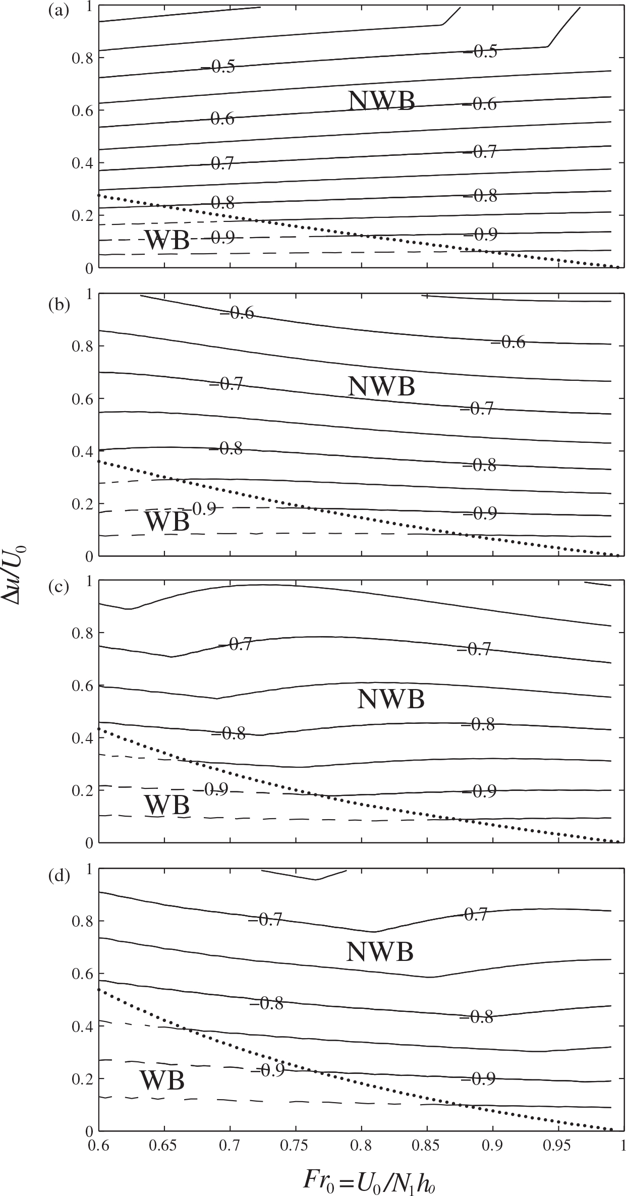
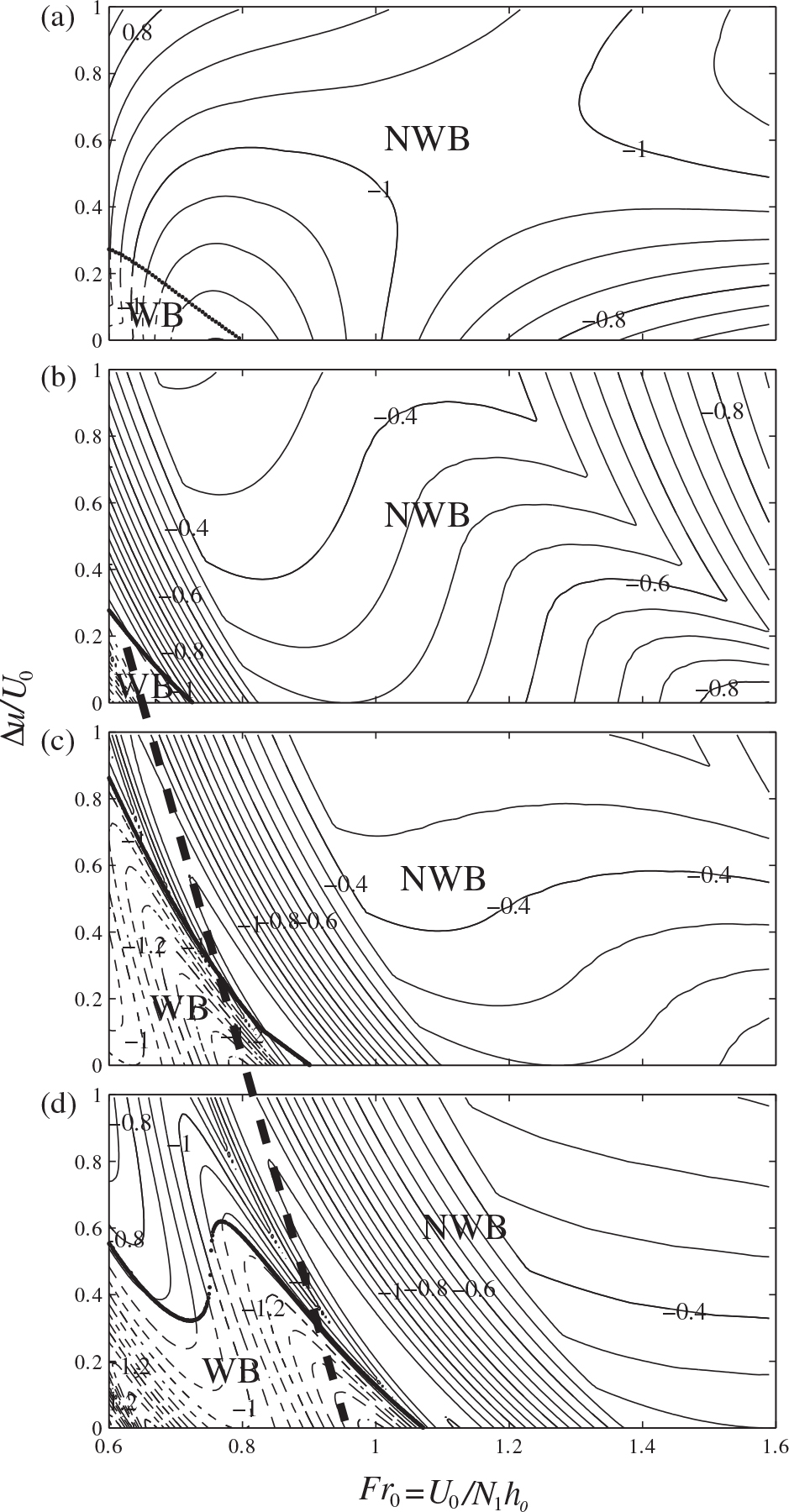
According to the parameter mapping method described above, the relationship between U 0 and Δu c is one-to-one matching, and Δu c decreases as U 0 increases. More details are given for Exps CTRL and B2 in Fig. 2. In addition, Fig. 3 depicts the non-dimensional maximum negative horizontal wind perturbation (MNHWP; u/N 1 h) depending on different values of Fr 0 and Δu/U 0, which indicates that the amplitude of topographic wave disturbance (solid contour) weakens rapidly with increasing Δu/U 0 (or Δu), but varies little with Fr 0 (or U 0); so for each U 0 over the range 0.6 ≤ Fr 0≤2.0, there would be a Δu that leads to a stagnation point where the total horizontal velocity is zero, and it is defined as Δu c. Meanwhile, if non-dimensionalising U 0 and Δu c obtained by the parameter mapping method (viz., Fr 0 and Δu c/U 0) and superimposing them onto Fig. 3, the orographic flow will be separated into two regimes: without GWB (NWB) and with GWB (WB), as shown by the dotted line in Fig. 3. Therefore, when U 0 is given, if Δu exceeds Δu c (viz. Δu>Δu c), there is no GWB's occurring over orography, which is in the NWB regime. Moreover, as shown in Fig. 3, Δu c decreases as U 0 increases over the range 0.6 ≤ Fr 0≤2.0; so there would be a maximum value of Δu c, denoted as MVWS (Δu max), and its corresponding surface wind speed (U 0) is labelled as U 0m, so in CTRL, Δu max=2.16 ms−1 and U 0m=0.6 N 1 h 0 (see Table 1 or Fig. 3b). This result implies that if the VWS is larger than MVWS (viz. Δu > Δu max), the GWB's occurring over orography will be suppressed, such as in CTRL; if Δu=3 ms−1>Δu max=2.16 ms−1, the orographic flow will have no GWB no matter what value U 0 has, as long as 0.6 ≤ Fr 0≤2.0. Therefore, it makes the flow regimes related to GWB in Lin and Wang (1996) unlikely in this situation. Similar to CTRL, in Exps B2 and B3 there is also Δu max (Table 1), and there will be no GWB over orography when Δu > Δu max. In a sense, this result confirms what were proposed by Smith (1989) that non-dimensional mountain height for wave breaking will increase with increasing low-level vertical shear and that if the VWS exceeds some critical value, there will be no GWB occurring.
Fig. 2.
Surface wind speed and its one-to-one correspondence to low-level VWS when the stagnation point starts appearing over the leeside in Exps CTRL (B1), B2, and B3. Dots, triangles, and asterisks denote Exps CTRL, B2, and B3, respectively.
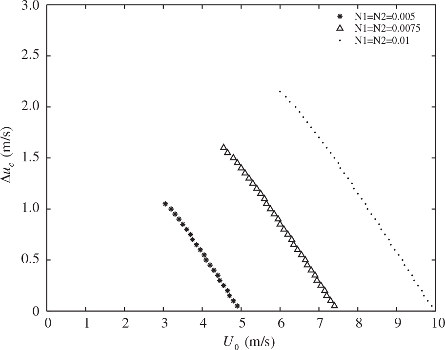
Fig. 3.
Normalised MNHWP (u/N 1 h) for different non-dimensional values of Fr 0 and Δu/U 0. The dotted line denotes the points for Fr 0 and the corresponding Δu c/U 0when the stagnation just appears over the leeside. ‘NWB’ denotes the region with no wave breaking (solid contour); ‘WB’ denotes the region with wave breaking (dashed contour). (a) Exp A1; (b) Exp CTRL; (c) Exp C1; and (d) Exp D1.
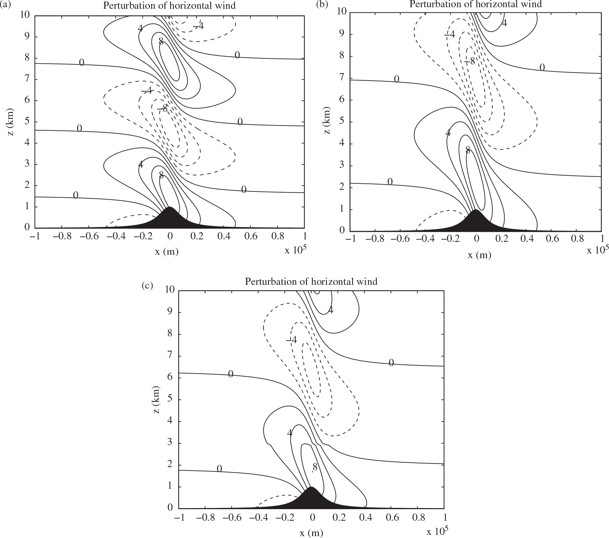
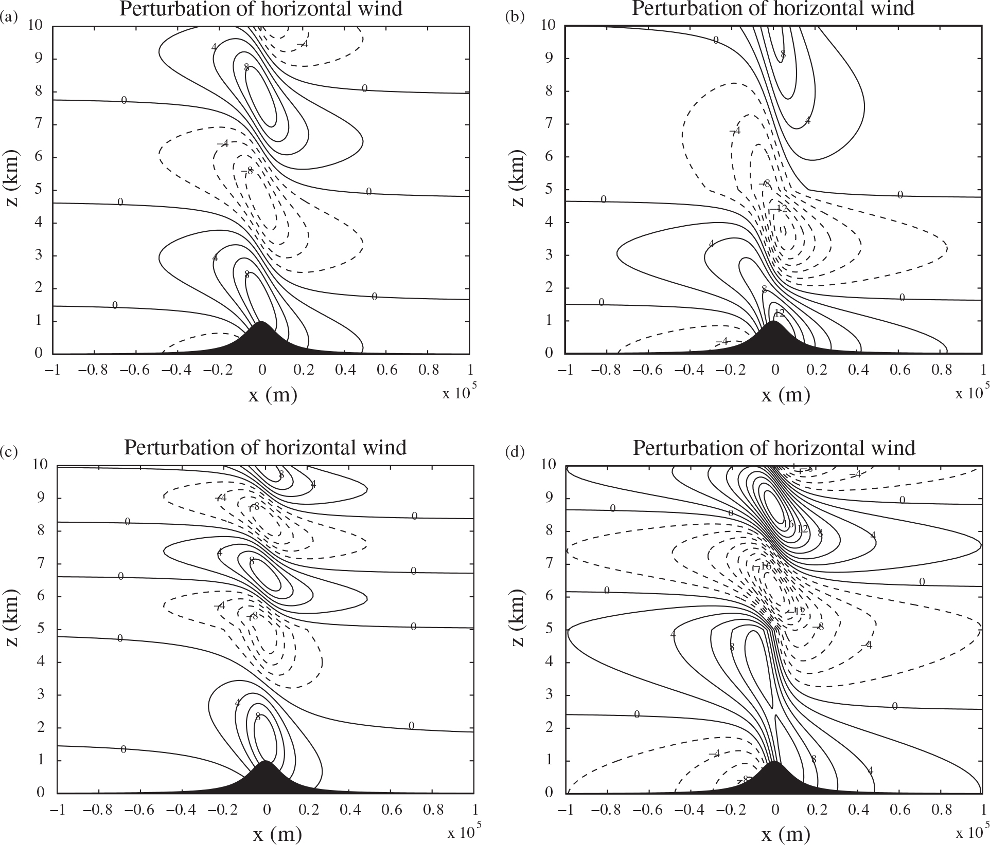
In order to verify the above statement that topographic wave disturbance weakens rapidly with increasing Δu, but varies little with U 0, the horizontal perturbation velocity in three different configurations for surface wind speed (U 0) and VWS (Δu) in CTRL is indicated in Fig. 4. Figures 4a,b illustrate there is slight variation in the amplitude of orographic disturbance for the uniform flow with different U 0 (here Δu≠0, but very small owing to the Richardson number introduced in this linear model). However, comparison of Fig. 4c with Fig. 4a shows that the negative perturbation of horizontal wind reduces rapidly with the increasing of Δu, which means that the orographic disturbance obviously weakens with the increasing of low-level VWS.
Fig. 4.
Horizontal perturbation velocity (contour interval of 2 ms−1) in CTRL with Δ=3 km and N 1=N 2=0.01 s−1. (a) U 0=10 ms−1, Δu=10−4 ms−1; (b) U 0=15 ms−1, Δu=10−4 ms−1; and (c) U 0=10 ms−1, Δu=5.0 ms−1.
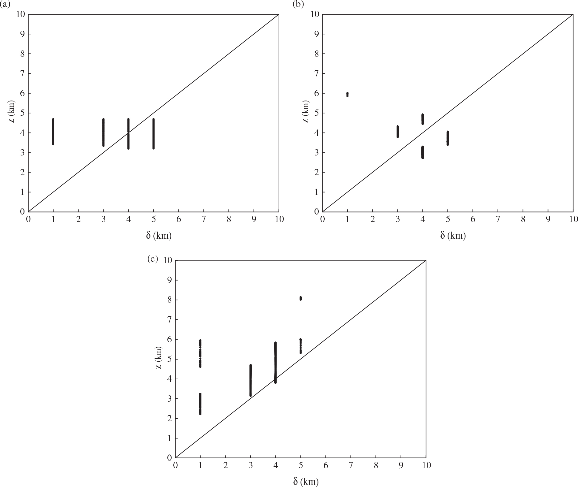
In addition, the lapse rate of orographic disturbance relative to Δu/U 0 (or Δu) increases as δ decreases, as shown in Fig. 3. That is because there is a larger VWS's effect to weaken orographic disturbance for shallower wind shear layer with the same Δu. And the maximum Δu/U 0 (Δu max/U 0m) is always at the same value of U 0/N 1 h 0 (especially, U 0/N 1 h 0=0.6) for each experiment in Case 1. Since h 0 is constant, that means U 0/N 1 is also constant. Therefore, if δ is given, there exists only one parameter (Δu/U 0) when wave breaking occurs, namely, Δu max/U 0m is a constant for a given Δ, when N 2/N 1=1 and no matter N 1=0.01, 0.0075 or 0.005 s−1, which can also be verified based on the numerical calculations in Table 1. Moreover, Δu max/U 0m (or Δu max) increases as Δ increases, and Exp D1 has the largest Δu max/U 0m=0.533 (or Δu max=3.2 ms−1); details are given in Table 1 and Fig. 5. Meanwhile, it is worth noting that the position of stagnation point begins in the upper layer (Exp A1), and shifts to that in the lower layer (Exp D1) as Δ increases (Fig. 6a).
Fig. 5.
Vertical configuration of the Brunt–Väisälä frequency (N 2/N 1) and corresponding Δu max/U 0m for different shear layer depth (Δ). Asterisks, hollow circles, crosses, and triangles denote Δ=1, 3, 4 and 5 km, respectively.
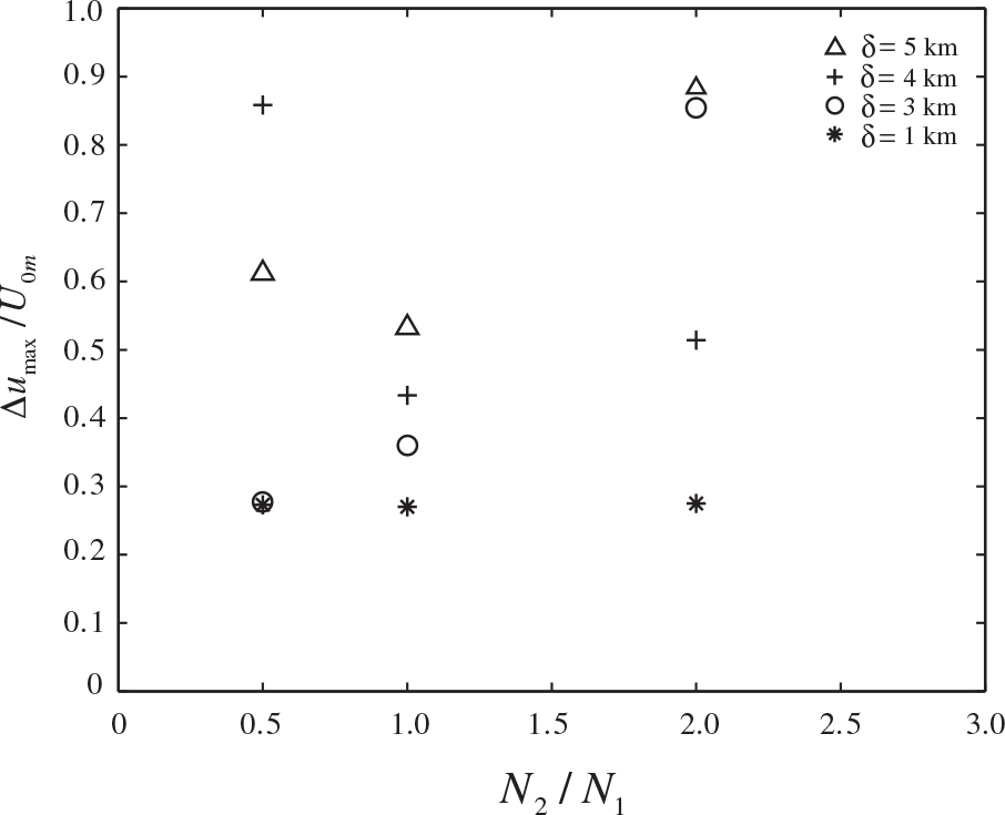
Fig. 6.
Vertical position of stagnation point (black point) calculated using the parameter-space search method. (a) Case 1 with N 2/N 1=1.0; (b) Case 2 with N 2/N 1=0.5; and (c) Case 3 with N 2/N 1=2.0.
3.2.2. Case 2:N2/N1=1/2.
Table 1 shows that there is also Δu max in Exps A4, B4 and C4 when U 0m=0.6 N 1 h 0, and Δu max also increases as Δ increases. However, Δu max is about 4.78 ms−1 in Exp D4, which is smaller than 5.15 ms−1 in Exp C4, and the surface wind speed U 0m=0.78×N 1 h 0. It is said that there exists another factor that limits the increase of Δu max except for the confinement of Fr 0≥0.6.
Skyllingstad (1991) identified that, if the atmospheric stability is not uniform in the vertical, there will be a layer interface between the lower and upper layers. This interface can induce wave reflection and resonance when the atmospheric stability above the interface is smaller, and the wave amplitude strengthened in the lower layer reduces with the increase of the ambient stability above the interface. When Δ/λ=1/4 + n/2 (n=0, 1, 2, …, and λ is vertical wavelength in the lower layer), the criteria for wave over-reflection proposed by Lindzen and Tung (1976, hereafter LT76) is even applicable to this situation. Based on LT76's criteria, the average thickness of the lower stable layer for the wave ducting is 1.8 km, which is calculated from the dispersion relation. Figure 7 displays the horizontal wind perturbation in Exps D1 and D4 with U 0=10 ms−1 and Δu=10−4ms−1. In Exp D1 with N 2/N 1=1, topographic wave can vertically propagation without wave reflection and ducting (Fig. 7a), but with N 2/N 1=1/2 in Exp D4, there is wave reflection at the layer interface between the lower and upper layers, and the wave amplitude below the interface is doubled (Fig. 7b). This result is consistent with the LT76's criteria on wave ducting, and it could explain why higher wind speed happened due to larger stability difference between upper and lower layers in the 1997 event than in 1999 event (Jones et al., 2002).
Fig. 7.
Same as in Fig. 4, but for: (a) U 0=10 ms−1, Δu=10−4 ms−1 in Exp D1; (b) U 0=10 ms−1, Δu=10−4 ms−1 in Exp D4; (c) U 0=10 ms−1, Δu=10−4 ms−1 in Exp D5; (d) U 0=16 ms−1, Δu=10−4 ms−1 in Exp D5.
Similar to the case of N 2/N 1=1, the orographic flow in Exps A4, B4, C4 and D4 have also two flow regimes: with GWB and without GWB (Fig. 8). And the non-dimensional MNHWP (u/N 1 h) also generally decreases as Δu increases, but its variation with Fr 0 becomes more remarkable than that in Case 1, because the vertical propagating gravity wave is reflected by the layer interface. Moreover, in Exps B4, C4 and D4 with Δ>1.8 km, the pattern of MNHWP tends to shift toward the cases with larger Fr 0 as Δ increases, as denoted by a broad dashed line in Fig. 8. The increase of Δ may enlarge the ducted vertical wavelength according to the LT76's criteria [λ=Δ/(1/4 + n/2)]. Based on U=λN/2π, the pattern of MNHWP will shift to the case with larger Fr 0 as Δ increases (Fig. 8). In addition, similar to the case of N 2/N 1=1, it can be found that Δu max/U 0m in the case of N 2/N 1=1/2 is also a constant when Δ is given (Figs. 5 and 8), and the stagnation point shifts from upper to lower layer as Δ increases (Fig. 6b).
Fig. 8.
As in Fig. 3, but: (a) Exp A4; (b) Exp B4; (c) Exp C4; and (d) Exp D4.
3.2.3. Case 3: N2/N1=2.
As shown in Fig. 9, the non-dimensional MNHWP varies with Fr 0 and Δu/U 0 in the case of N 2/N 1=2. The distribution of MNHWP also shifts to the case with larger Fr 0 from Exp B5 to Exp D5. However, the features of topographic waves in this case are different from those in Case 2. In Case 3 the amplified topographic wave exists in the upper layer: there is no obvious variation of wave amplitude in the vertical transmission process when Δ/λ=1/4 + n/2, such as in Exp D5 when U 0=10 ms−1, Δu = 10−4 ms−1 (Fig. 7c). When Δ/λ=n/2, however, the gravity wave amplitude in the upper layer is doubled, such as in Exp D5 when U 0=16 ms−1, Δu = 10−4 ms−1 (Fig. 7d).
Fig. 9.
As in Fig. 3, but: (a) Exp A5; (b) Exp B5; (c) Exp C5; and (d) Exp D5.
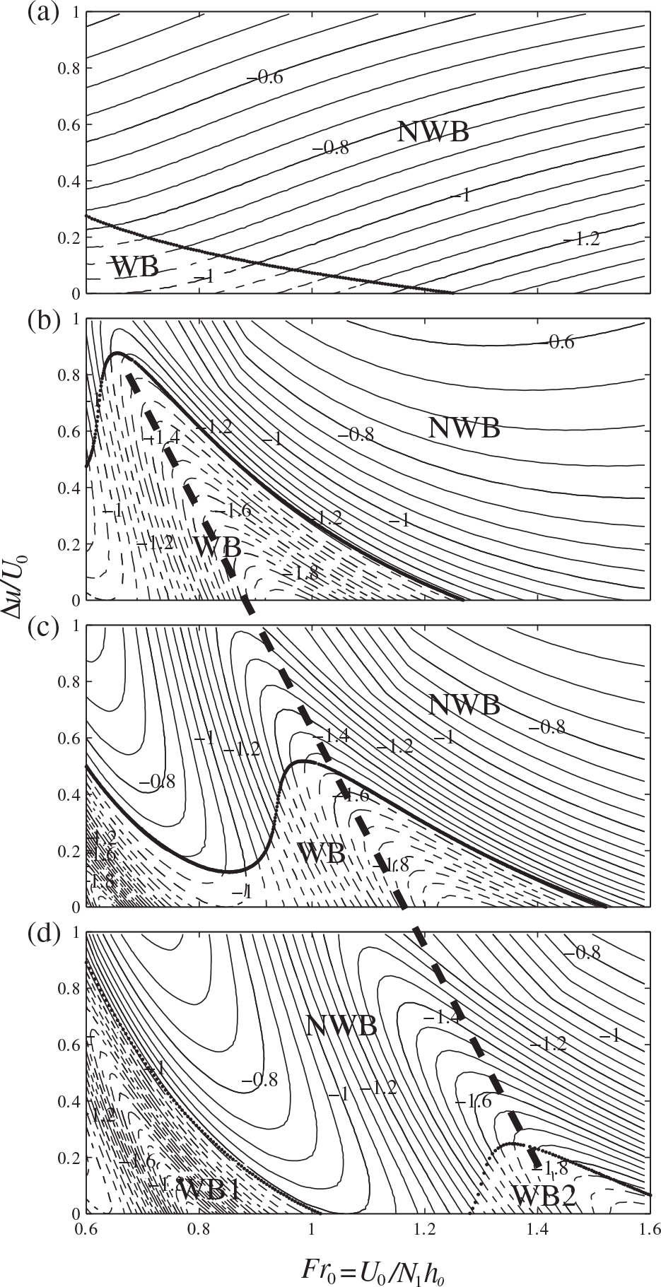
Moreover, there are two subzones (WB1 and WB2) for the GWB in Exp D5. In WB1 (0.6 ≤ Fr 0≤1.02), Fr 0 is a relatively small and there is Δu max=5.3 ms−1 when Fr 0=0.6. In WB2 (1.28 ≤ Fr 0≤1.69), the features are the same as those in WB1, but Δu max=3.5 ms−1, which is smaller than 5.3 ms−1 in WB1. Additionally, when 1.02 < Fr 0<1.28 or Fr 0>1.69, there will be no stagnation point in this area because MNHWP is smaller than the basic wind speed (not shown).
As displayed in Fig. 5, Δu max/U 0m in Case 3 is also a constant for a given Δ, similar to Cases 1 and 2, though only in Case 1 Δu max/U 0m increases with increasing Δ. It is also worth noting that Δu max/U 0m of Exp B5 (Δ=3 km, N 2/N 1=2, Δu max/U 0m=0.854) is almost equal to that of Exp C4 (Δ=4 km, N 2/N 1=1/2, Δu max/U 0m=0.858), which means Δu max/U 0m may have the same value in different cases with different Δ as long as the Brunt–Väisälä frequency configuration is adjusted in both lower and upper layers. In Case 3, however, almost all the stagnation points are located in the upper layer, which is different from those in Cases 1 and 2 (Fig. 6c).
In summary, over the range of 0.6 ≤ U 0/N 1 h 0≤2.0, when there exists a low-level VWS layer, no matter what the Brunt–Väisälä frequency profile is, there will be a maximum critical VWS (Δu max) for GWB's occurring over orography. If the low-level VWS Δu > Δu max, the flow over orography will not generate GWB.
3.3. Discussion
Based on the two-layer linear model, the effects of VWS on mountain wave disturbance were investigated. The amplitude of wave rapidly weakens as the VWS increases, so there exists a maximum critical VWS Δu max for GWB's occurring, and when the VWS Δu > Δu max, GWB will not occur.
The above results are obtained based on the linear theory, however, so these results may be influenced by inherent limitations of the linear theory. For example, in a single-layer linear model with constant N and U, Lilly and Klemp (1979) have identified that the wave amplitude is roughly similar between linear theory and finite-amplitude solution for a small terrain, but the assumption of constant N and U can play a role to restrain non-linear responses of gravity wave (Smith, 1977). Furthermore, as discussed in Durran (1986, 1992) the non-linear effect sharply strengthens as the mountain height increases, and the linear theory predicts a weak response where large-amplitude wave is produced for a larger mountain height, so that the horizontal wind perturbation in a linear model may be smaller than that in the reality, and then there may exist some deviations on the estimation of critical VWS (Δu c ) obtained between the linear model and the real atmosphere. Besides, in a multilayer linear model of orographic flow with different atmospheric stability, the dependence of wave response prediction is different on stability profile. Based on the demonstrations by Durran (1992), when the higher stability is in the lower layer (as in Case 2 of N 2/N 1=1/2), the real wave response increases as the mountain height increases, which means that the linear model could underpredict the wave response, and then Δu c may be overpredicted by the linear theory for a larger mountain height. In addition, the real wave response is sensitive to the location of the stability interface when the higher stability is located in the upper layer (Durran 1992), e.g. when the interface is at the height of 0.5 λ, the linear theory predicts a stronger wave response, and then Δu c will be underpredicted by the linear theory. However, when the interface is at the height of 0.6 λ, the wave response predicted by the linear theory is significantly weaker than that in the reality, so Δu c is overpredicted by the linear theory. Thus, in the present study the critical VWS (Δu c) may be overpredicted in Case 1 (N 2/N 1=1) and Case 2 (N 2/N 1=1/2), and underpredicted in some experiments of Case 2 (N 2/N 1=1/2). Moreover, since there are two factors controlling the VWS profile, namely, the height of interface (Δ) and VWS increment (Δu), the prediction error of (Δu c) from the VWS profile mainly depends on the height of interface. Therefore, the accuracy of the calculation for Δu c depending on the shear profile is similar to that on the stability profile. Of course, this present study only discussed the case of constant low-level VWS. Therefore, the study on more accurate calculation of Δu c is needed to go beyond the linear theory in the future.
4. Concluding remarks
Two-dimensional, steady-state, non-rotating, frictionless, two-layer linear model of orographic flow with a low-level VWS is developed to study flow dynamics over an isolated orography. Using the analytical solutions derived from this linear model, the effects of the VWS on GWB's occurring over orography were discussed. However, all results discussed in the present study are confined over the range of 0.6 ≤ U 0/N 1 h 0≤2.0 in order to exclude the impact of upstream blocking to the formation of GWB. If the orographic height (h 0), atmospheric stability parameters (N 1 and N 2), and the height of VWS layer (Δ) are given, the horizontal surface basic wind (U 0) and its one-to-one corresponding critical VWS (Δu c) for GWB's occurring can be determined by a parameter-space search. Therefore, if U 0 is also given, when the VWS (Δu) is larger than its critical VWS (Δu c), i.e. Δu > Δu c, the occurring of GWB over orography will be suppressed.
In addition, over the selected range of surface Froude number (Fr b≤Fr 0≤Fr d), there is a maximum critical VWS (Δu max) within Δu c and a relative surface wind speed (U 0m) for the occurring of GWB. It implies that, if Δu > Δu max, there will be no GWB's occurring over orography no matter what value U 0 has, as long as 0.6 ≤ U 0/N 1 h 0m≤2.0. Therefore, the flow regimes related to GWB's occurring in the case of uniform upstream flow proposed by Lin and Wang (1996) will disappear when the low-level VWS is larger than a critical one. It also confirms Smith's hypothesis that non-dimensional mountain height for wave breaking will increase with increasing VWS, and exceeds some value, there will be no GWB. Moreover, if Δ and N 2/N 1 are constant, Δu max/U 0m will also be a constant.
Why does there exist a MVWS for GWB's occurring over orography? Firstly, in the regimes for higher surface Froude number, MNHWP is smaller than the basic horizontal wind, which is the same as that in a uniform upstream flow. Secondly, MNHWP generally decreases as VWS increases.
Furthermore, the response of Δu max to atmospheric stability configuration in the lower and upper layers is different. When N 2/N 1=1, the variation of MNHWP in response to U 0 is weak, and rapidly decreases with increasing Δu; so Δu c reaches a maximum value at U 0=0.6 N 1 h 0. When N 2/N 1=1/2 or 2, owing to different Brunt-Väisälä frequencies in the lower and upper layers, the vertically propagating gravity wave may be amplified or diminished by reflection from the layer interface, which leads to its distribution pattern shifting to a higher Froude number as Δ increases, and U 0m also shifts to a higher Froude number, maybe no longer at U 0=0.6 N 1 h 0, such as in Exps C5 and D4.
Since the present study adopts two-layer linear model to investigate the impact of VWS on mountain waves and GWB, the errors of prediction in wave response are included due to the limitations of the linear theory (Durran, 1986, 1992). Compared with that in the real atmosphere, consequently, the critical VWS (Δu c) obtained in this study might have deviations depending on some factors, i.e. larger mountain height, stability and VWS profile as discussed in Section 3. Nevertheless, it seems true that the amplitude of topographic wave weakens as VWS increases; so there should exist a maximum value of Δu max, and if Δu > Δu max, the GWB does not occur, which was quantitatively proved in this study. Maybe it is helpful to understand the response of topographic flow on low-level VWS. In addition, a non-linear model may be needed to further investigate the VWS's effect on GWB.
5. Acknowledgements
This research is supported by the National Natural Science Foundation of China through the grants 40921160381, 41130964 and 41005033, and by the National Special Funding Project for Meteorology (GYHY201006004). The authors are grateful to Dr. Wang Qi Wei for discussions and constructive comments on our initial results, and greatly appreciate the valuable comments from the anonymous reviewers, which greatly improved the presentation of this paper.