Fig. 1.
MM5 control forecast from 00 UTC 9 June to 06 UTC 11 June 2000 initialised using ECMWF 24-h forecasts. (Left) Potential vorticity on the 330 K isentropic surface (dashed line, in PV units), sea level pressure (continuous line, in hPa) and 6-h accumulated rainfall (shaded contours, in mm according to scale) on (a) 9 June at 18 UTC and (c) 10 June at 00 UTC. (Right) Water vapour flux convergence in the 1000–700 hPa (continuous line, contour interval is 1 g−2 s–1, starting at 1 g−2 s−1), convective instability (as measured by the equivalent potential temperature difference between 1000 and 500 hPa, at intervals of 5 °C starting at 5 °C; dashed line) and precipitable water (shaded contours, in mm according to scale) on (b) 9 June at 18 UTC and (d) 10 June at 00 UTC.
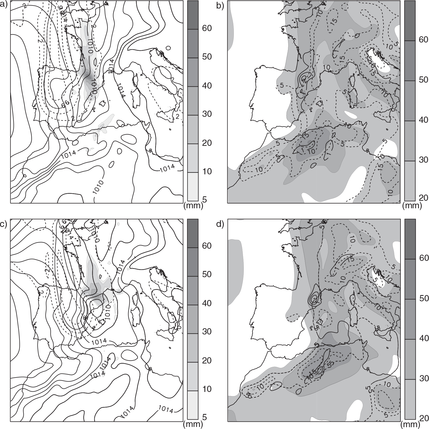
Fig. 2.
Comparison of MM5 control forecast against ECMWF analyses for the June 2000 event. (Left) Potential vorticity on the 330 K isentropic surface (dashed line, in PV units) and sea level pressure (continuous line, in hPa) on (a) 9 June at 18 UTC and (c) 10 June at 00 UTC, according to the analyses. (Right) Differences between the corresponding MM5 control forecast and the analyses for the potential vorticity on the 330 K isentropic surface (shaded contours plain/patterned for positive/negative values, in PV units according to scale) and sea level pressure (continuous/dashed line for positive/negative values, in hPa) on (b) 9 June at 18 UTC and (d) 10 June at 00 UTC.
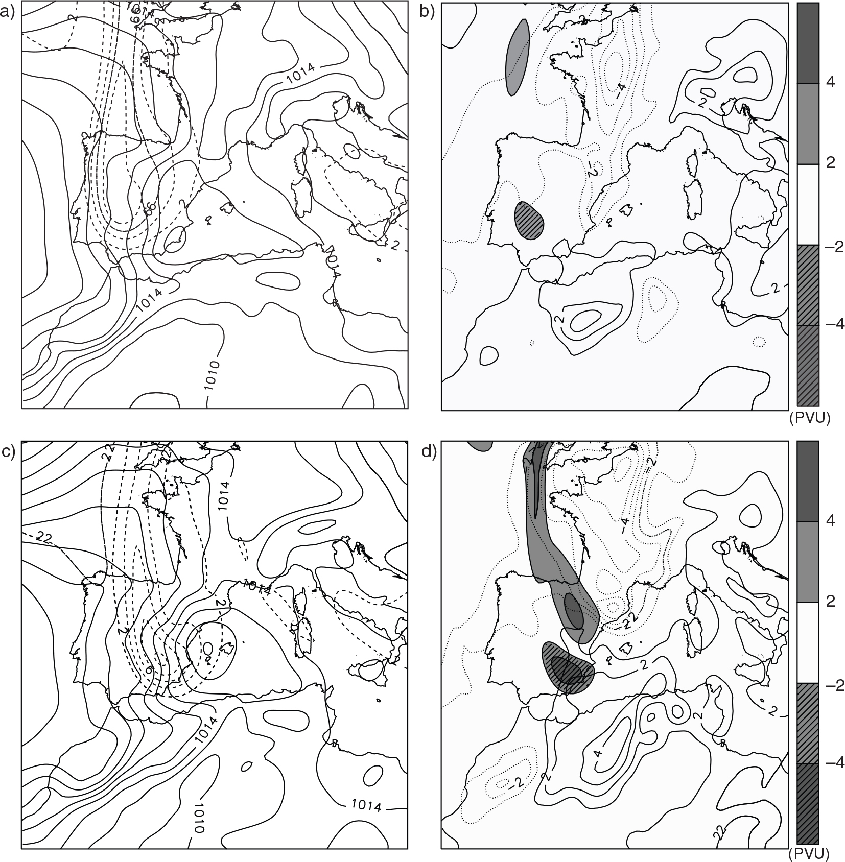
Fig. 3.
Same fields as shown in Fig. 1, except for the MM5 control forecast from 00 UTC 9 October to 06 UTC 11 October 2002. (a and b) 9 October at 18 UTC and (c and d) 10 October at 00 UTC. The arrows in (b) and (d) denote the position and direction of the low-level jet (LLJ).
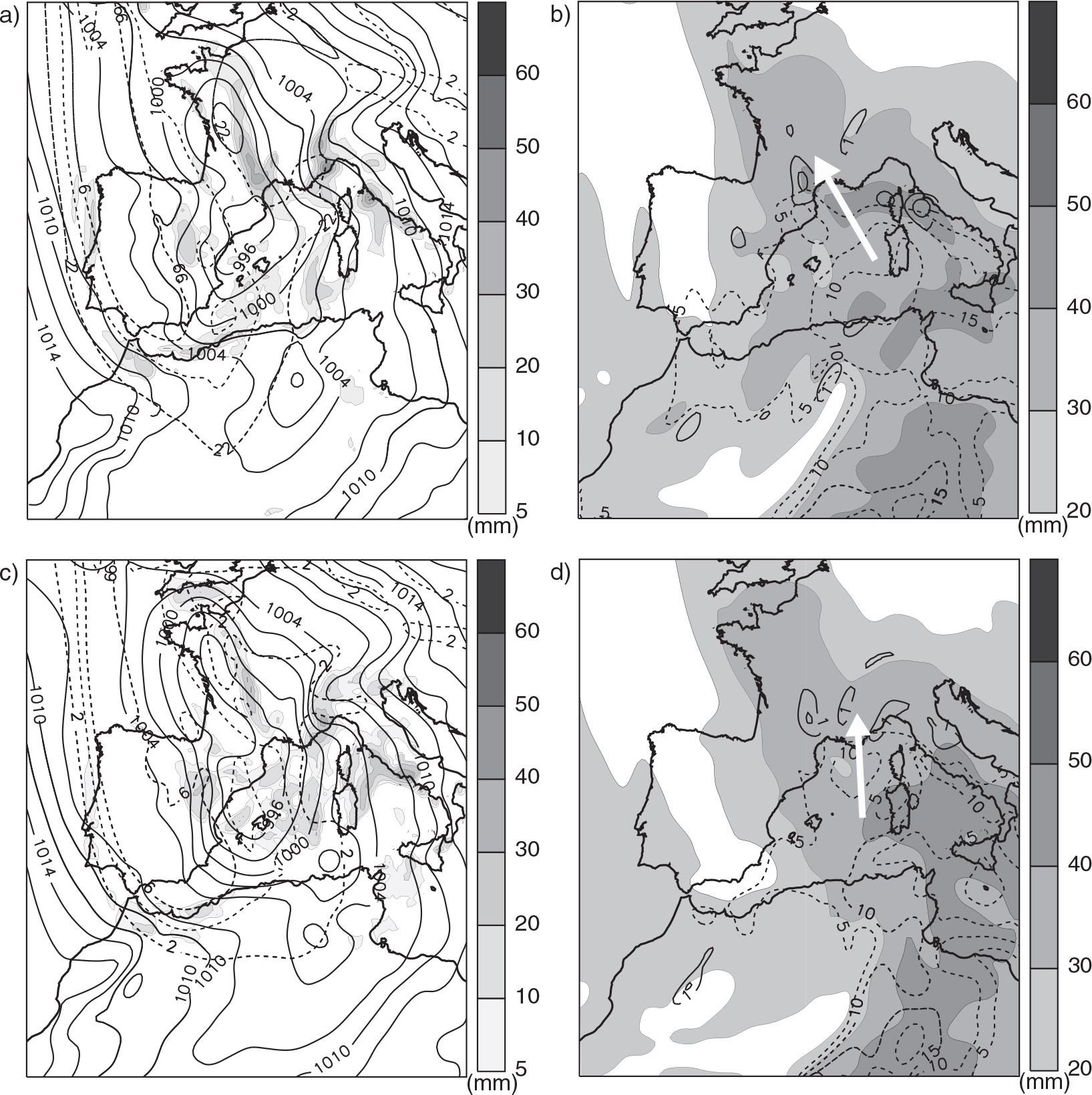
Fig. 4.
Same fields as shown in Fig. 2, except for the October 2002 event. (a and b) 9 October at 18 UTC and (c and d) 10 October at 00 UTC.
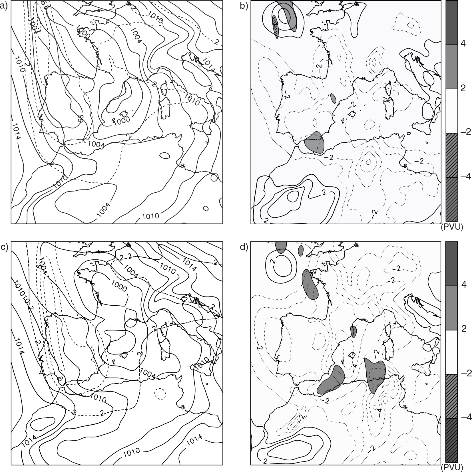
Fig. 5.
Overlay for 9 June 2000 at 00 UTC of the potential vorticity field at 300 hPa unperturbed and perturbed (solid and dashed lines, respectively, contour interval 2 PVU, above 4 PVU) and METEOSAT-7 water vapour brightness temperatures (shading, in K according to scale). The letters G and C indicate the locations where the PV modifications are applied (see the details in the text).
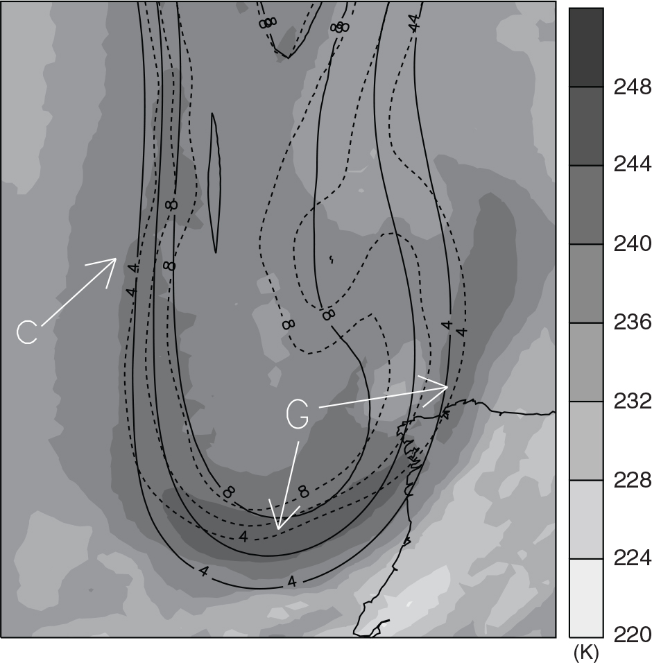
Fig. 6.
MM5 perturbed forecast, once the potential vorticity modifications are applied, from 00 UTC 9 June to 06 UTC 11 June 2000. (Left) Potential vorticity on the 330 K isentropic surface (dashed line, in PV units), sea level pressure (continuous line, in hPa), and 6-h accumulated rainfall (shaded contours, in mm according to scale) on (a) 9 June at 18 UTC and (c) 10 June at 00 UTC. (Right) Differences between the MM5 perturbed forecast and the corresponding MM5 control forecast (shown in Fig. 1) for the potential vorticity on the 330 K isentropic surface (shaded contours plain/patterned for positive/negative values, in PV units according to scale) and sea level pressure (continuous/dashed line for positive/negative values, in hPa) on (b) 9 June at 18 UTC and (d) 10 June at 00 UTC.
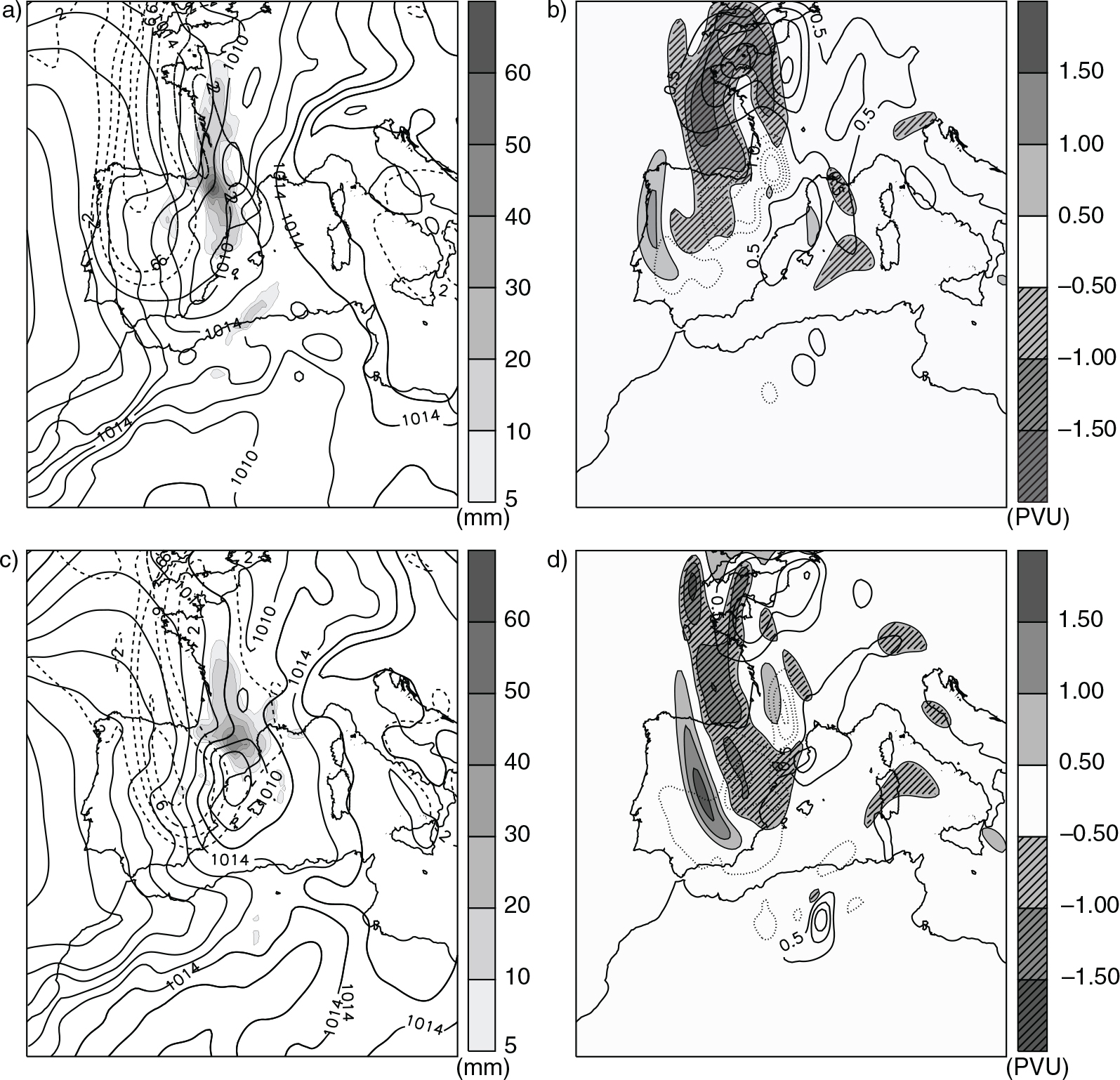
Fig. 7.
Same fields as shown in Fig. 6, except for the October 2002 event. (a and b) 9 October at 18 UTC and (c and d) 10 October at 00 UTC.
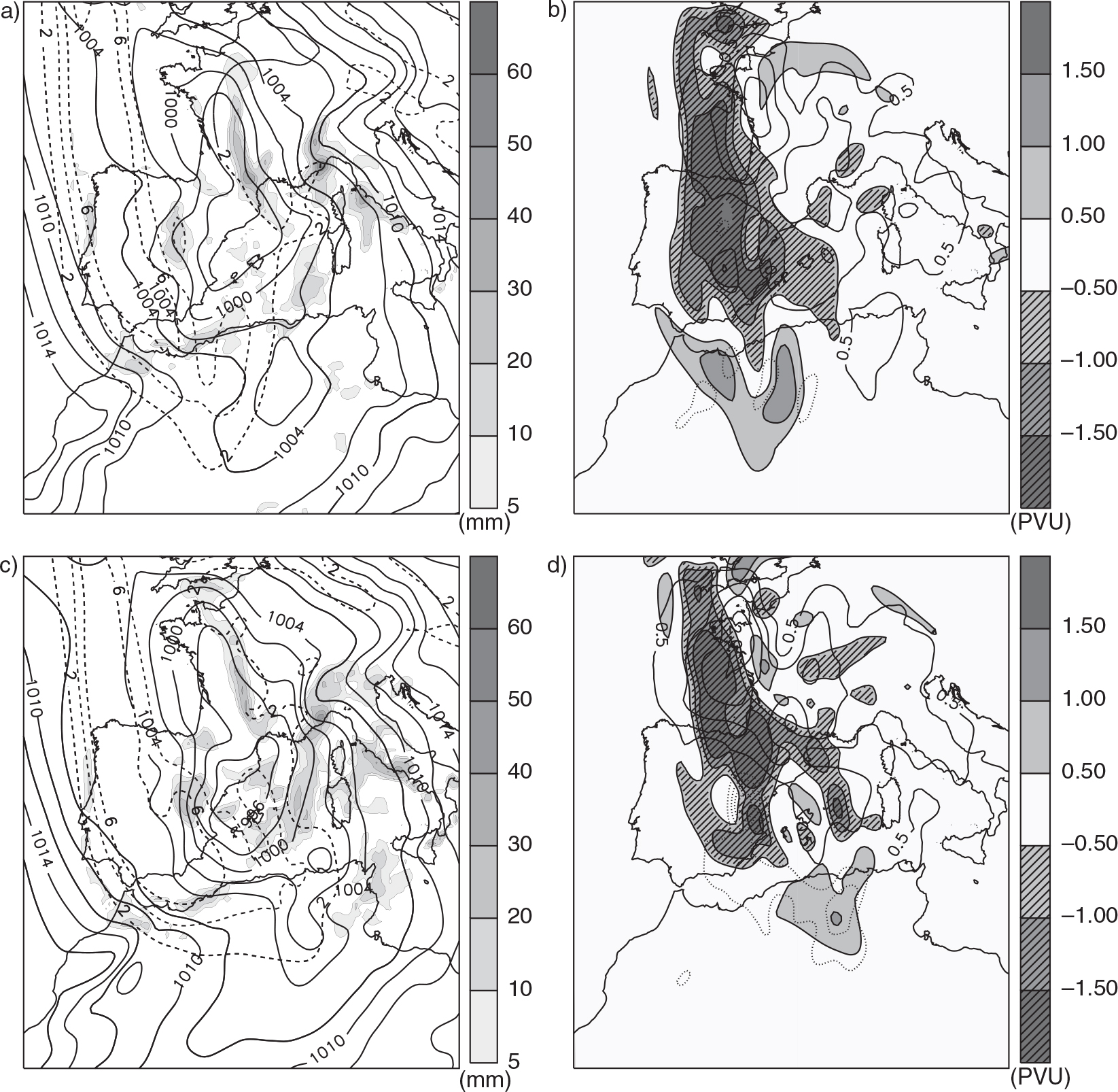
Fig. 8.
Accumulated rainfall (shaded, in mm according to scale) between 10 June 2000 at 06 UTC and 11 June 2000 at 06 UTC. (a) Non-perturbed run, (b) PV-WV run and (c) observed.
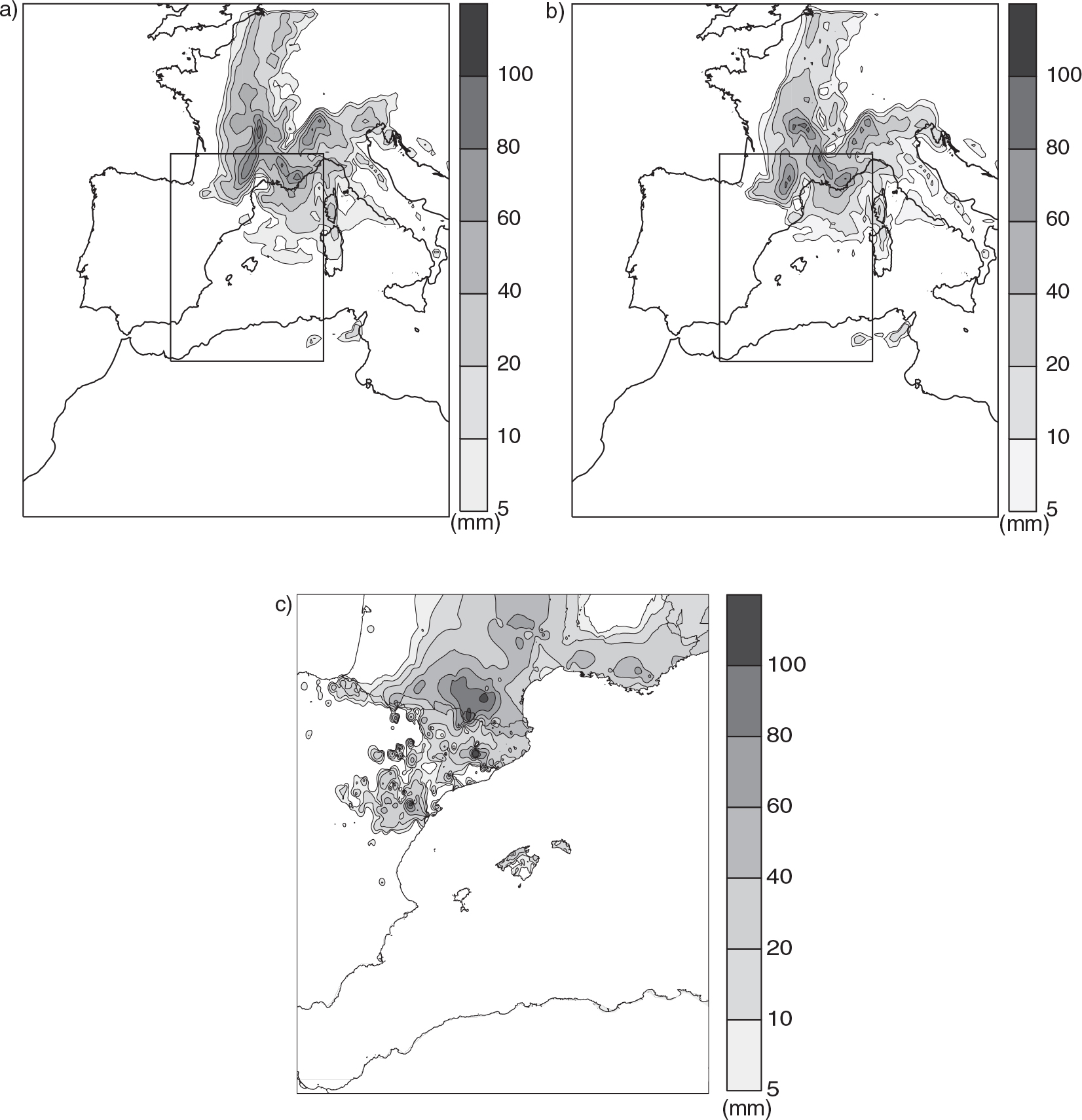
Fig. 9.
Accumulated rainfall (shaded, in mm according to scale) between 10 October 2002 at 06 UTC and 11 October 2002 at 06 UTC. (a) Non-perturbed, (b) PV-WV run and (c) observed.
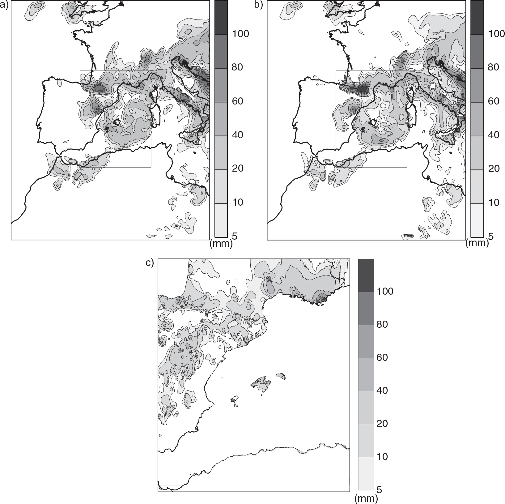
Fig. 10.
ROC area range for the PV-gradient and PV-adjoint ensemble members, where the empty square corresponds to the non-perturbed run and the filled square to the PV-WV perturbed run. (a) June 2000 event and (b) October 2002 case. The vertical lines represent these ROC area ranges where the extremes, maximum and minimum, of the range correspond to the ensemble member associated with the highest/lowest value of ROC area.
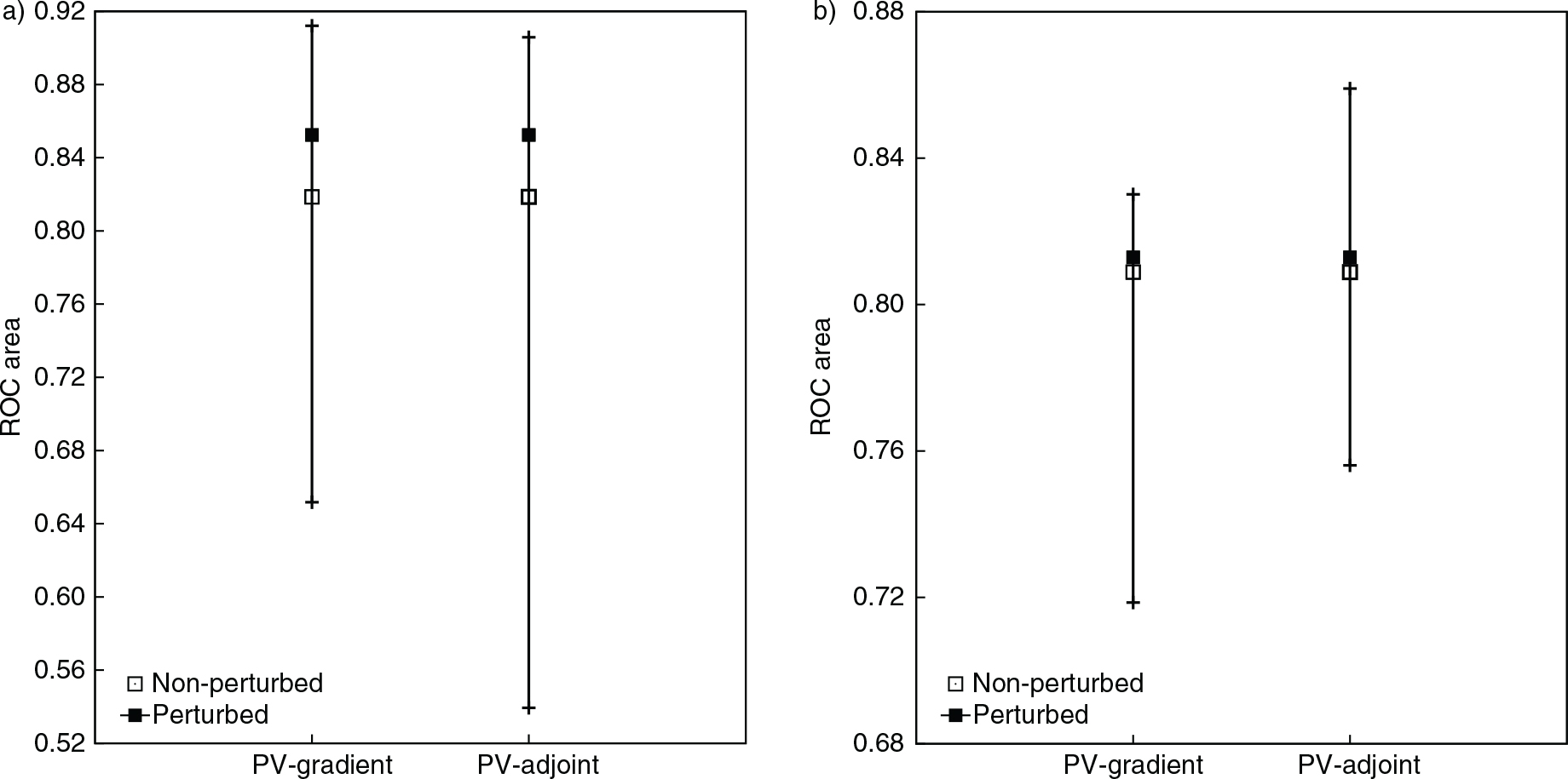
Fig. 11.
Q-Q plot for the PV-gradient and PV-adjoint ensemble members, where the dashed line corresponds to the non-perturbed run and the dotted line to the PV-WV perturbed run. (a) June 2000 event and (b) October 2002 case.
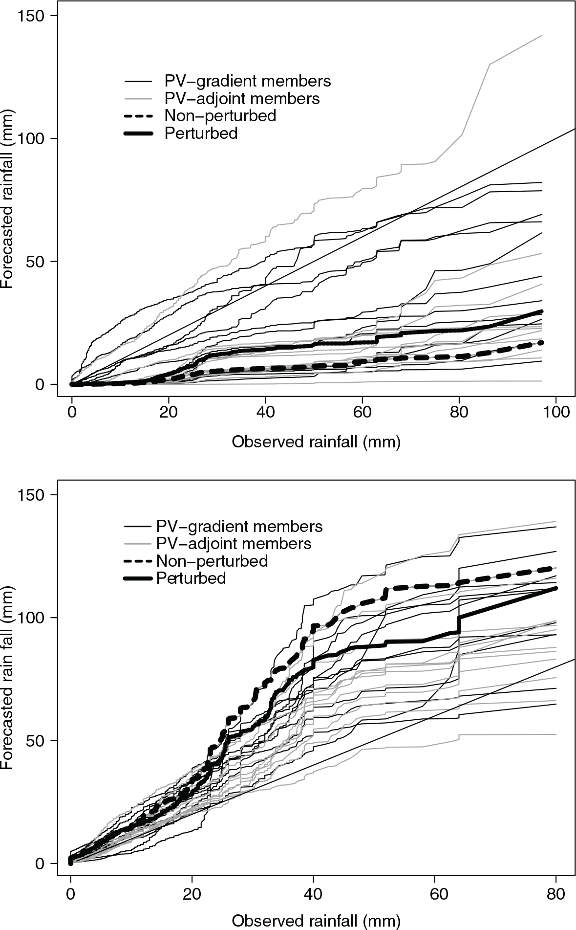
Fig. 12.
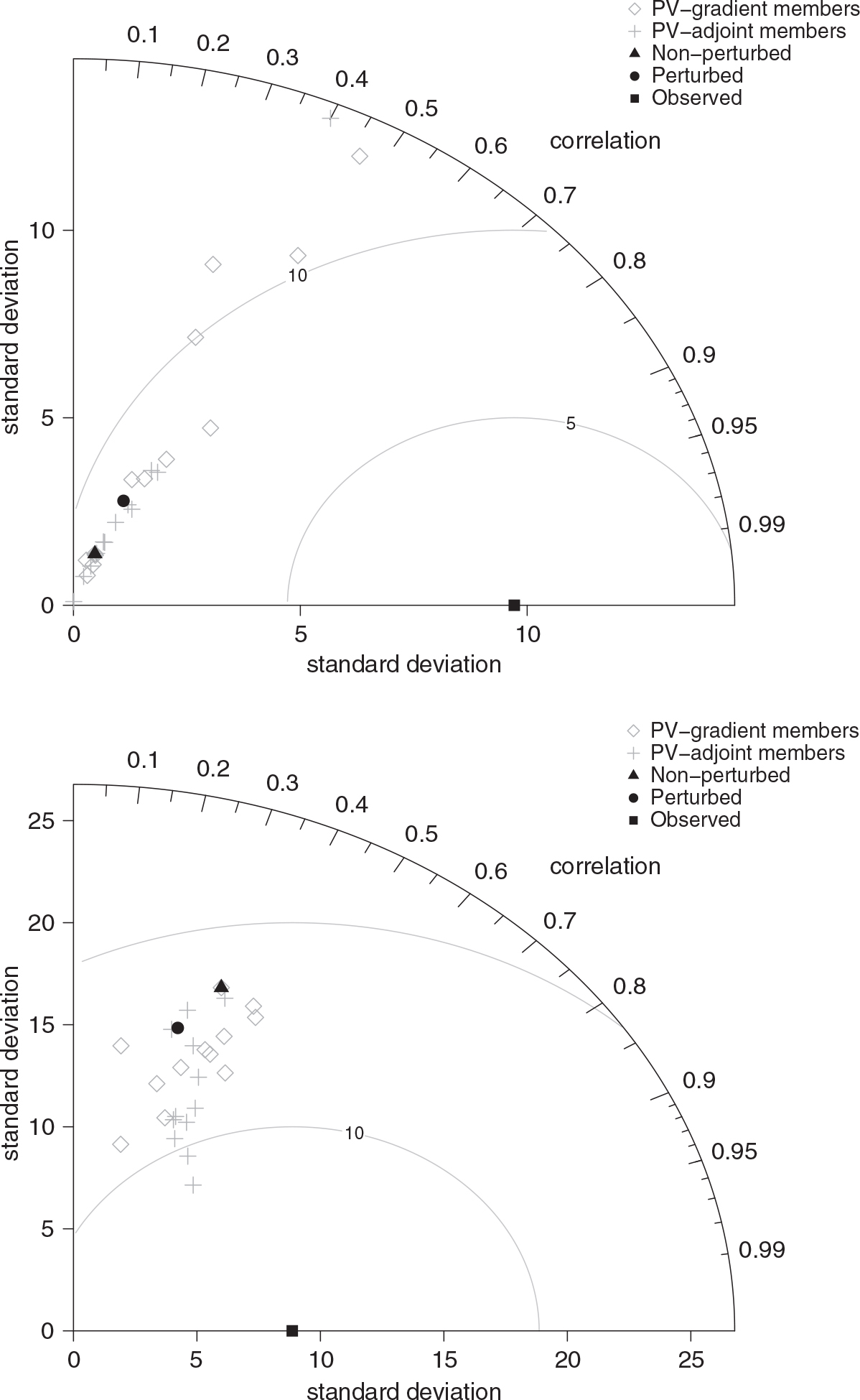
Taylor diagram for the PV-gradient and PV-adjoint ensemble members, where the solid triangle corresponds to the non-perturbed run, the solid circle to the PV-WV perturbed run and the solid square to the observations. (a) June 2000 event and (b) October 2002 case. The radial distance from the origin is proportional to the standard deviation of a pattern. The centred RMS difference between the observed and forecast field is proportional to their distance apart. The correlation between the two fields is given by the azimuthal position of the forecast field. The standard deviation and centred RMS difference units are rainfall in millimetres. The perfect score is obtained when the data point representing the forecast field matches up with the observed one.