Fig. 1.
The entire simulation domain comprising 170×158 grid points, and the outer 20 grid point halo and nesting zones. The lake fraction (in%) and lake depths (m) are shown. The blue arrows show locations of lakes used for evaluation of simulations and presented in Figs 2–13 and Table 1. The dashed contour denotes the lake-rich region of the domain, shown in Figs 14–19.
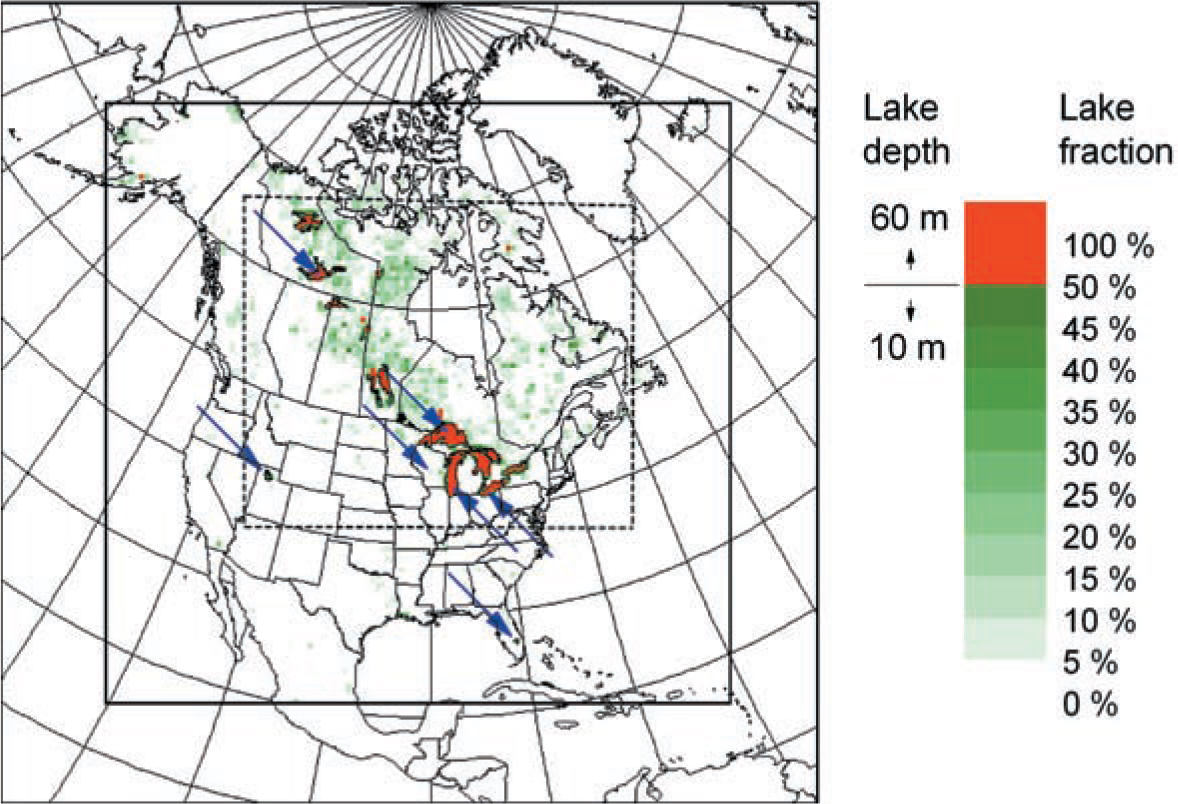
Table 1. Lake evaluation sites: characteristics and data sources
Fig. 2.
Comparison of simulated lake surface temperatures with MODIS-derived values for Great Slave Lake, Northwest Territories.
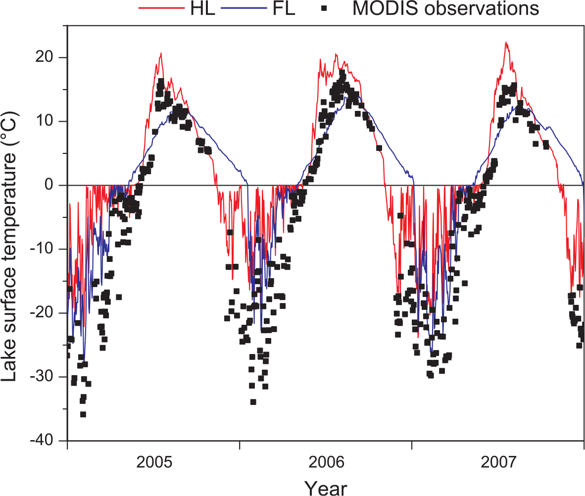
Fig. 3.
Comparison of simulated lake surface temperatures with buoy observations for Lake Superior.
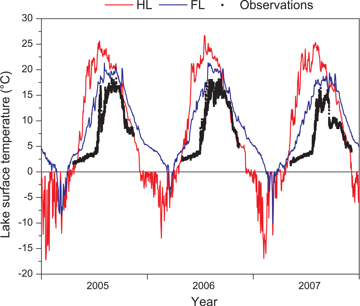
Fig. 4.
Same as Fig. 3, but for Lake Michigan.
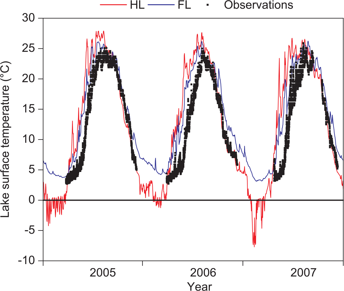
Fig. 5.
Same as Fig. 3, but for Lake Erie. FL-depth: simulated lake surface temperature, obtained with realistic lake depth parameterisation (20 m at the lake Erie buoy location).
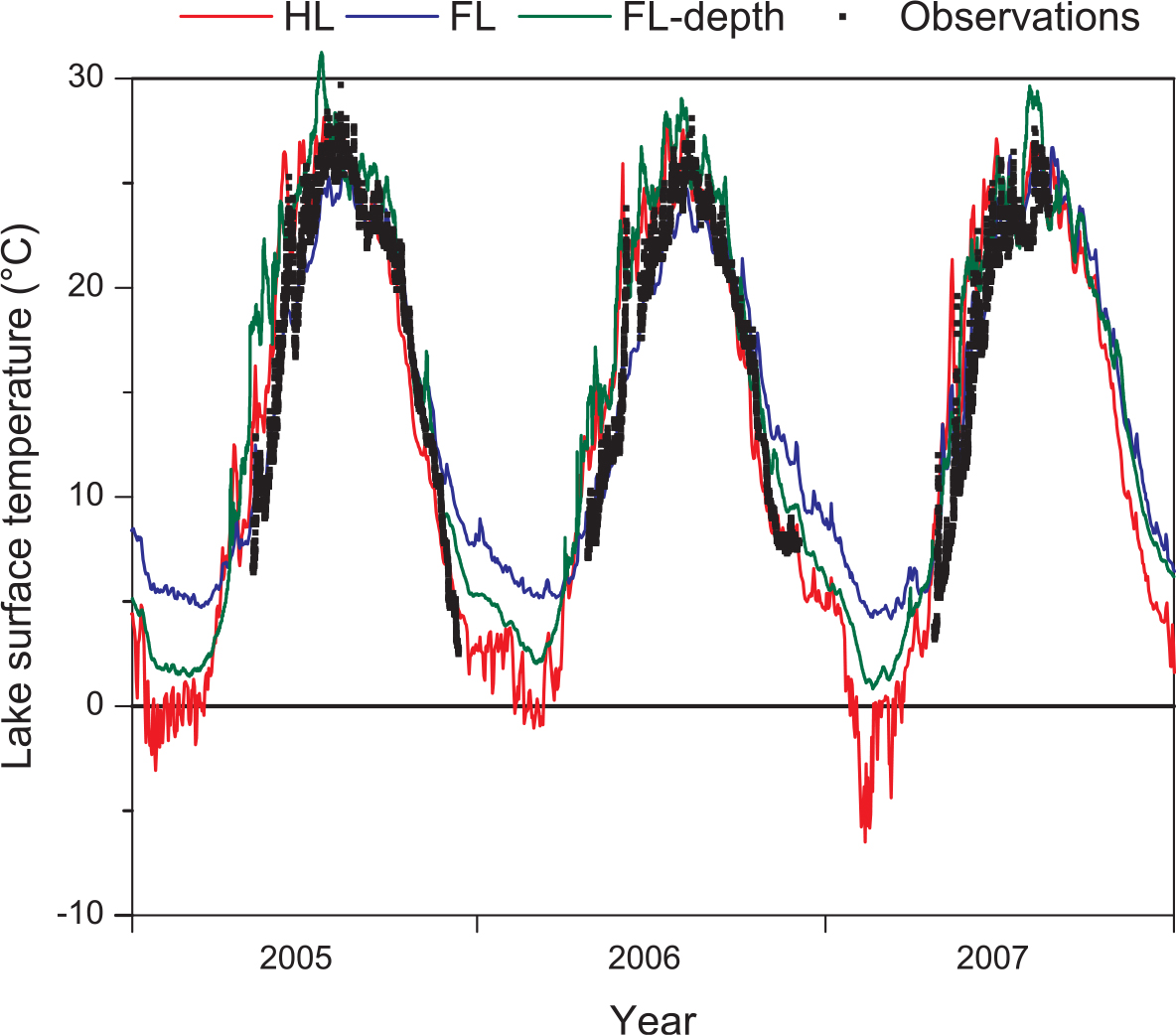
Fig. 6.
Same as Fig. 3, but for Sparkling lake, Wisconsin.
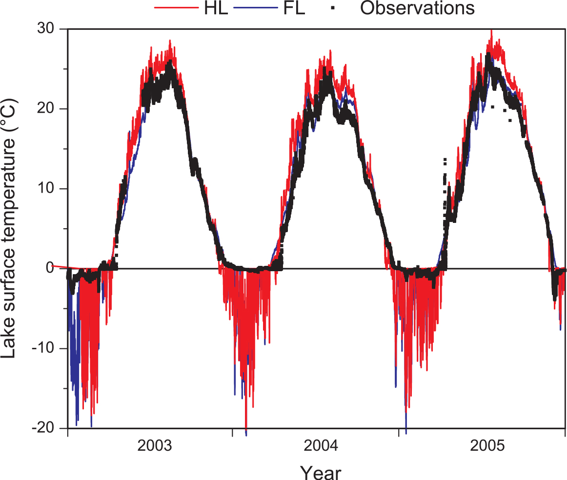
Fig. 7.
Same as Fig. 3, but for Great Salt Lake, Utah.
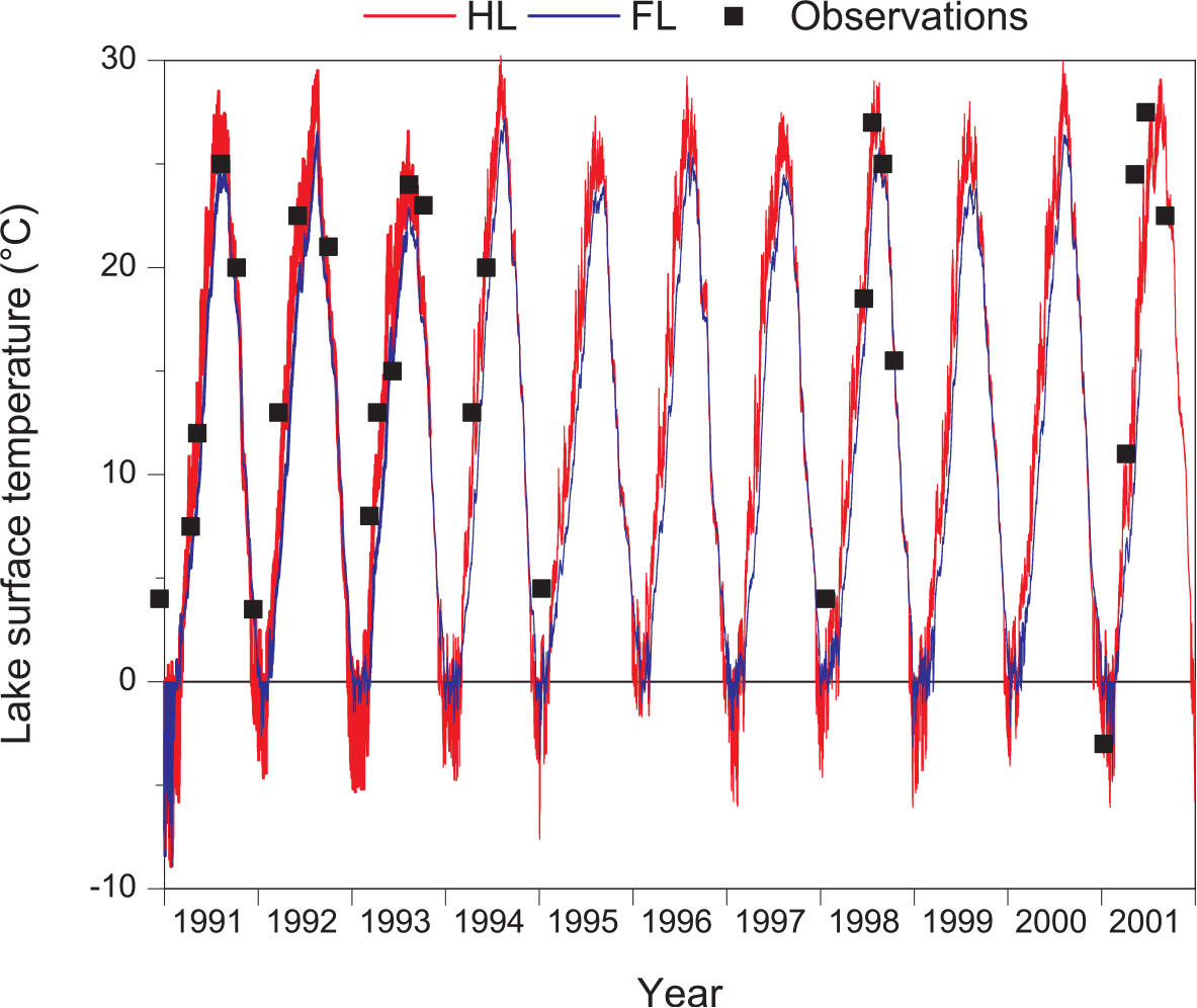
Fig. 8.
Same as Fig. 3, but for Lake Okeechobee, Florida.
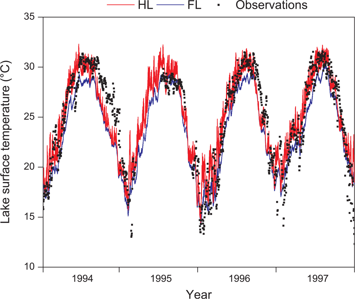
Fig. 9.
Annual cycle of simulated fields for Great Slave Lake, by the no-lake (NL) and the two coupled-lake (HL and FL) simulations, averaged over the 30-year period 1973–2002. The following fields are shown: screen-level temperature (upper left panel, in °C), screen-level specific humidity (upper right panel, in g kg−1), difference between the surface and screen-level air temperatures (middle left panel, in °C), difference between the surface and screen-level specific humidity (middle right panel, in g kg−1), surface sensible heat fluxes (lower left panel, in W m−2) and surface latent heat fluxes (lower left panel, in W m−2). Solid symbols denote absolute values, open symbols – differences.

Fig. 10.
Same as Fig. 9, but for Lake Superior.
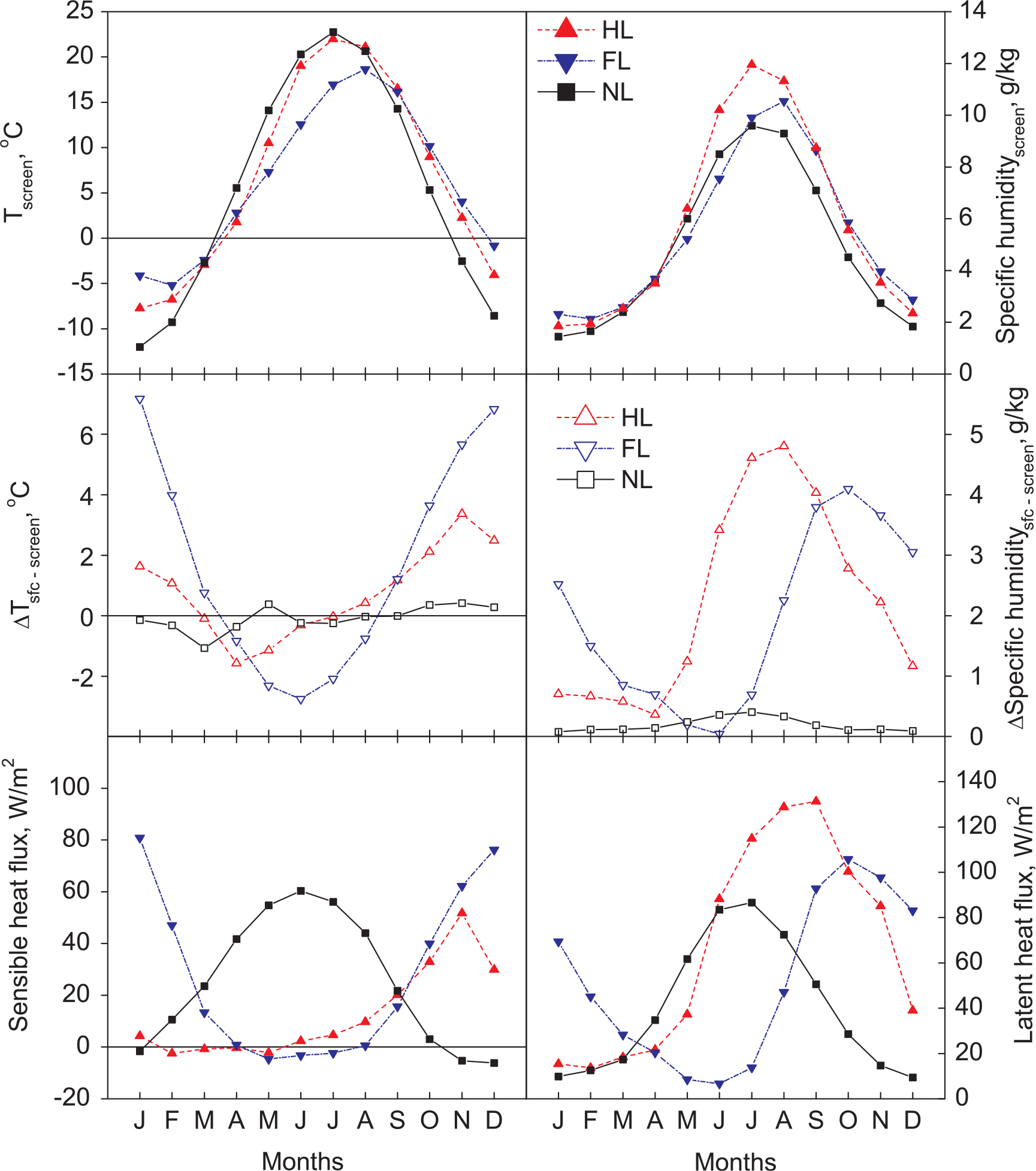
Fig. 11.
Same as Fig. 9, but for Lake Sparkling.
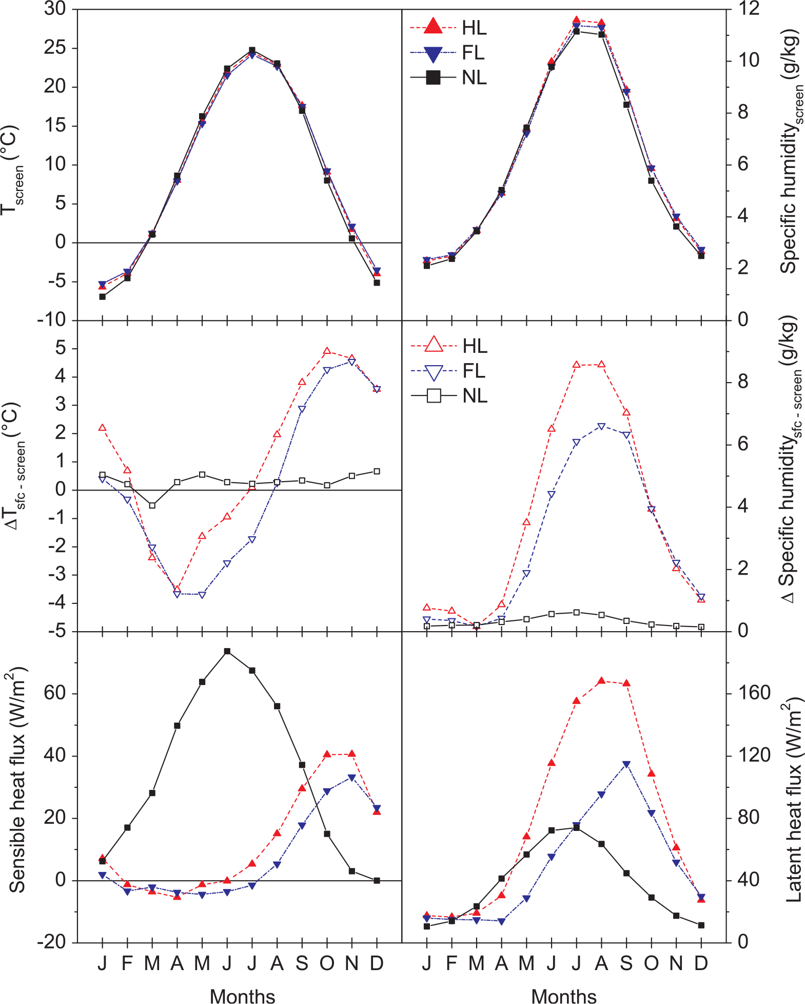
Fig. 12.
Same as Fig. 9, but for Great Salt Lake.
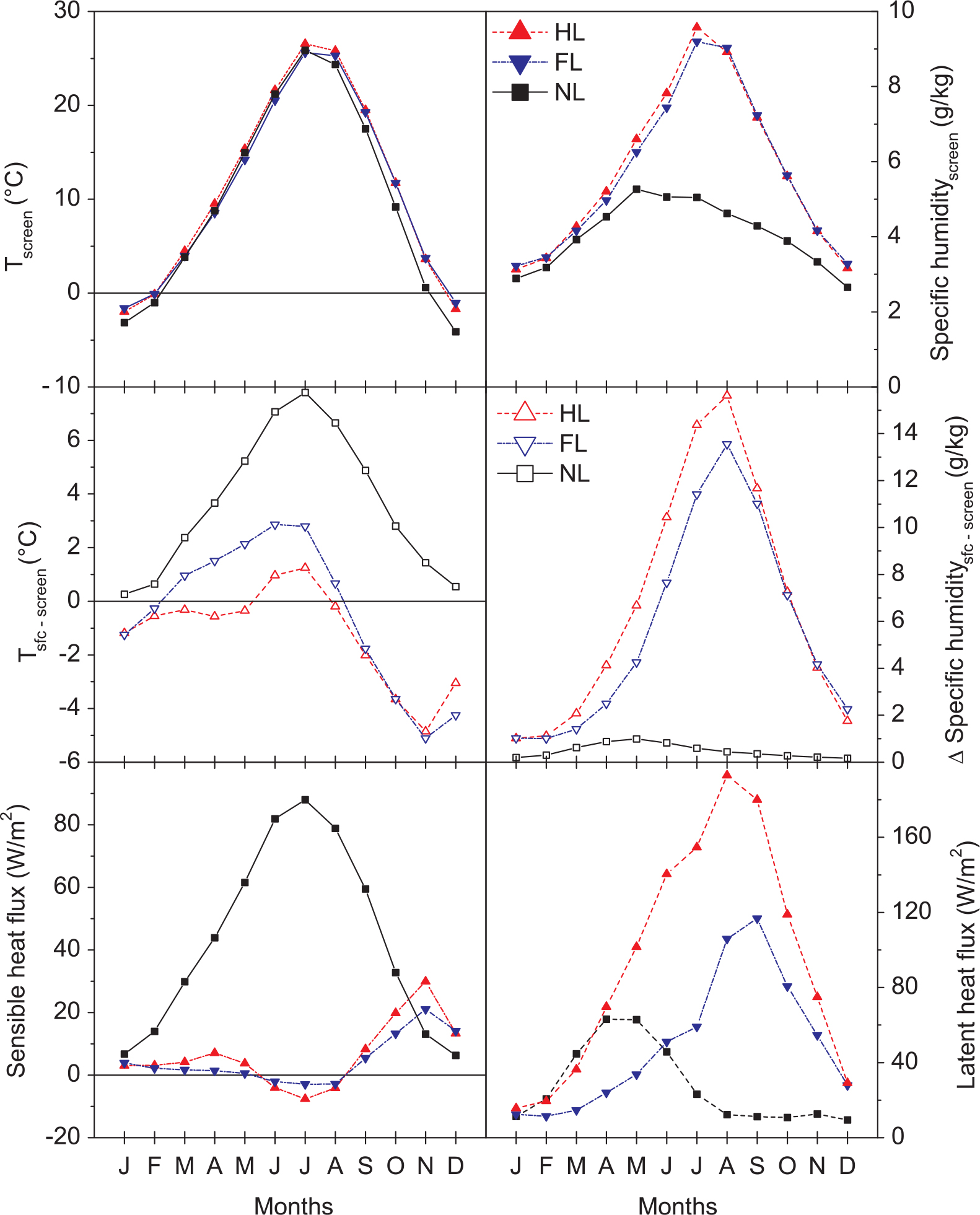
Fig. 13.
Same as Fig. 9, but for Lake Okeechobee.
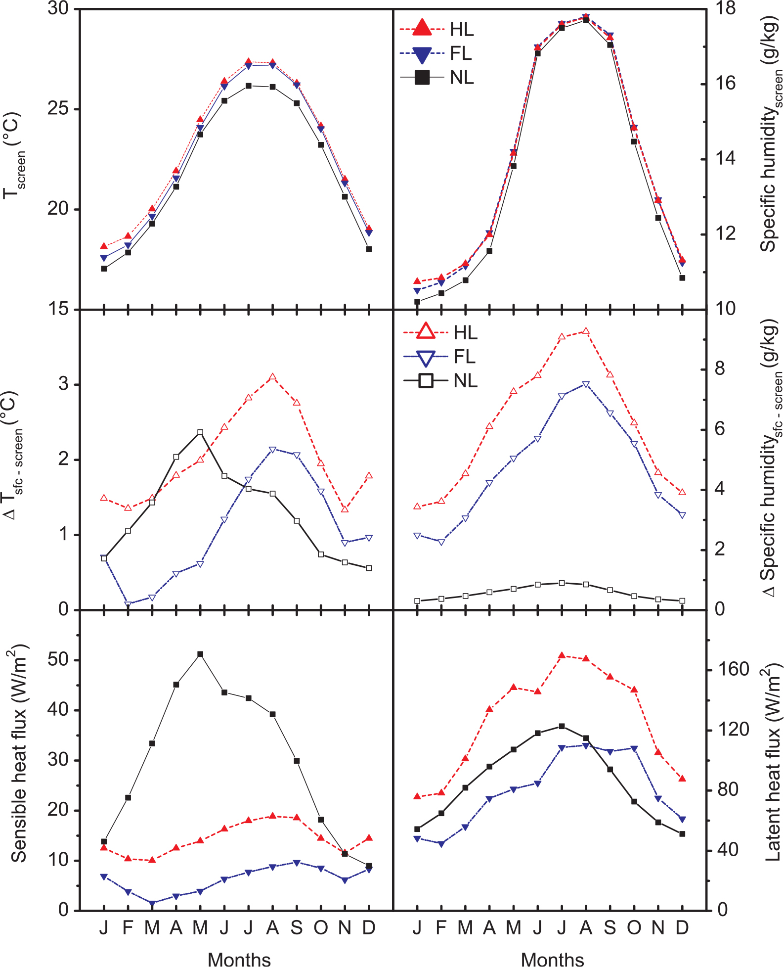
Fig. 14.
Screen-level temperature (in °C) climatological maps for 1973–2002, by ‘seasons’: spring (MAM), summer (Summer (JJA)), autumn (Autumn (SON)) and winter (Winter (DJF)). Top row corresponds to the NL simulation, second row to the reference CRU gridded analysis of observations, third row to the NL-simulation bias calculated as the difference between the NL simulation and the reference, fourth row to the difference between the HL and NL simulations and fifth row to the difference between the FL and NL simulations. Results are only shown over the continent, and the differences are only shown where statistically significant at the 95% level.
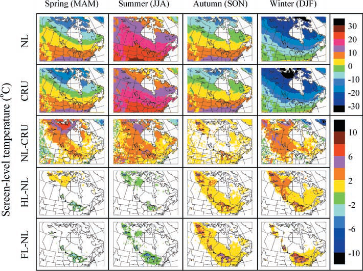
Fig. 15.
Climatological maps for 1973–2002 of screen-level specific humidity (in g kg−1). Top row corresponds to the NL simulation, second row to the difference between the HL and NL simulations and third row to the difference between the FL and NL simulations. Results are only shown over the continent and where the differences are statistically significant at the 95% level.
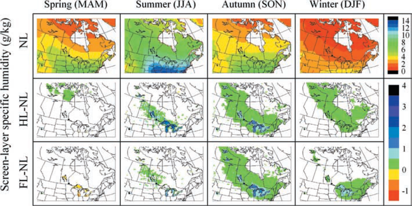
Fig. 16.
Same as Fig. 15, but for relative humidity (in%).
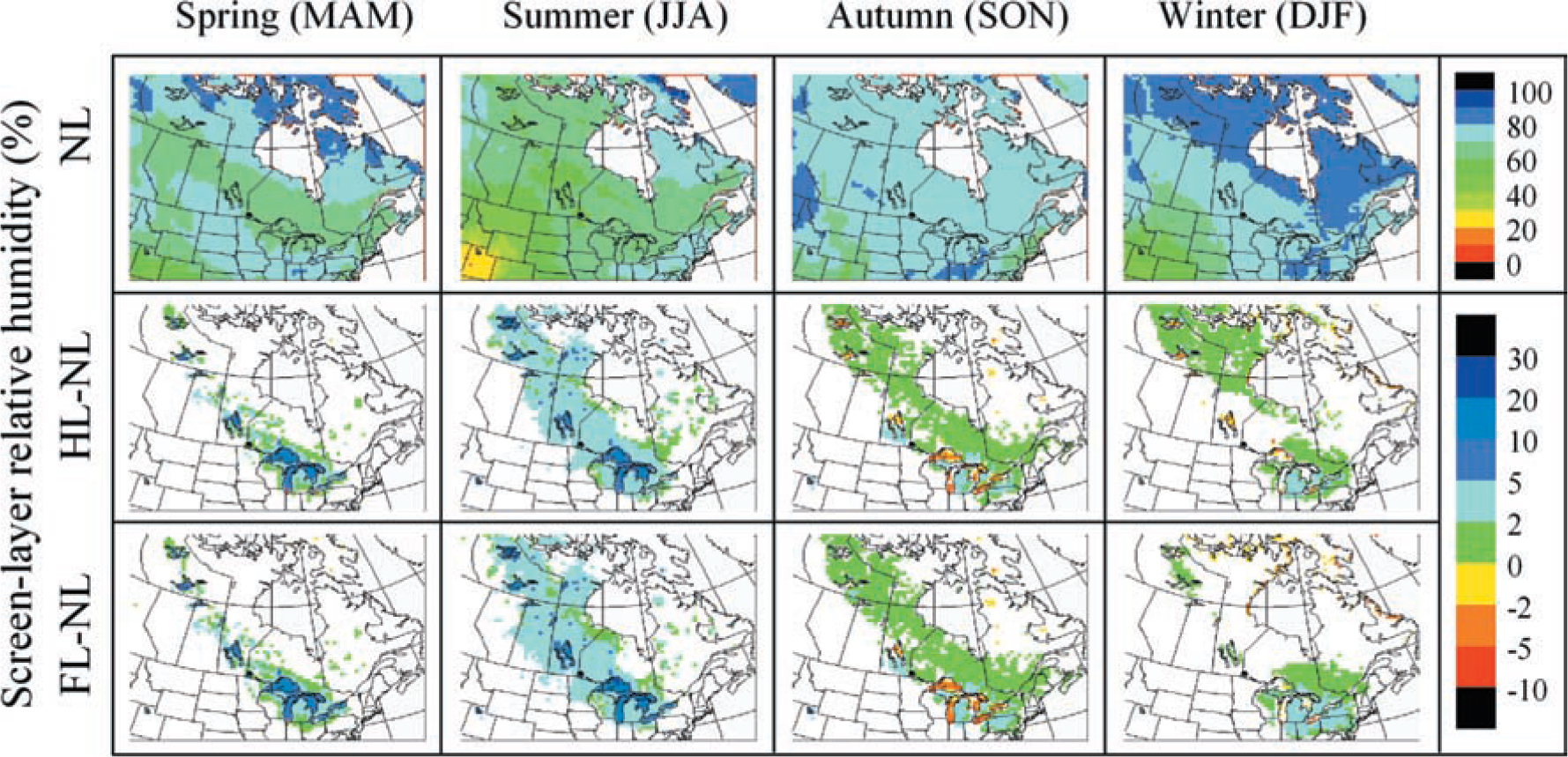
Fig. 17.
Same as Fig. 15, but for surface sensible heat flux (in W m−2). In this case, the ERA40 data are used as reference.
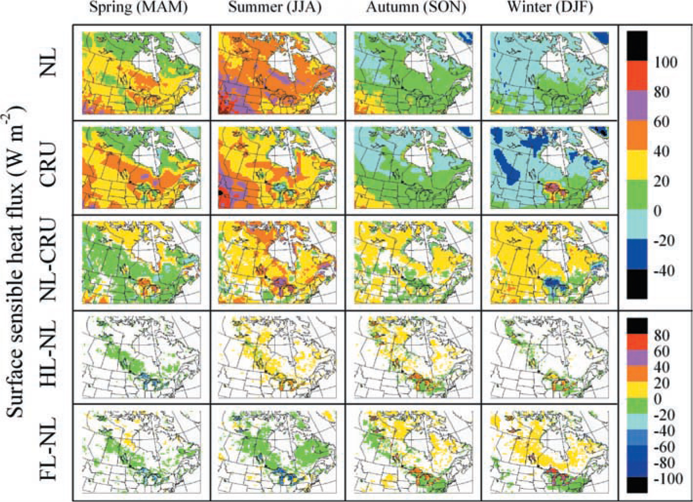
Fig. 18.
Same as Fig. 17, but for surface latent heat flux (in W m−2).
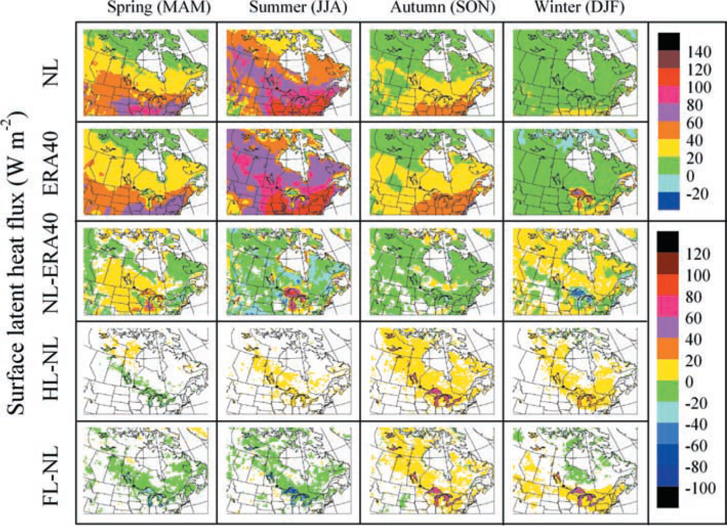
Fig. 19.
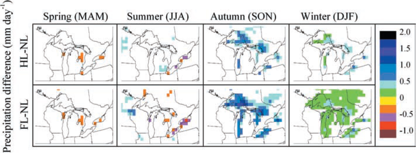
Same as Fig. 15, but for precipitation (in mm day−1).
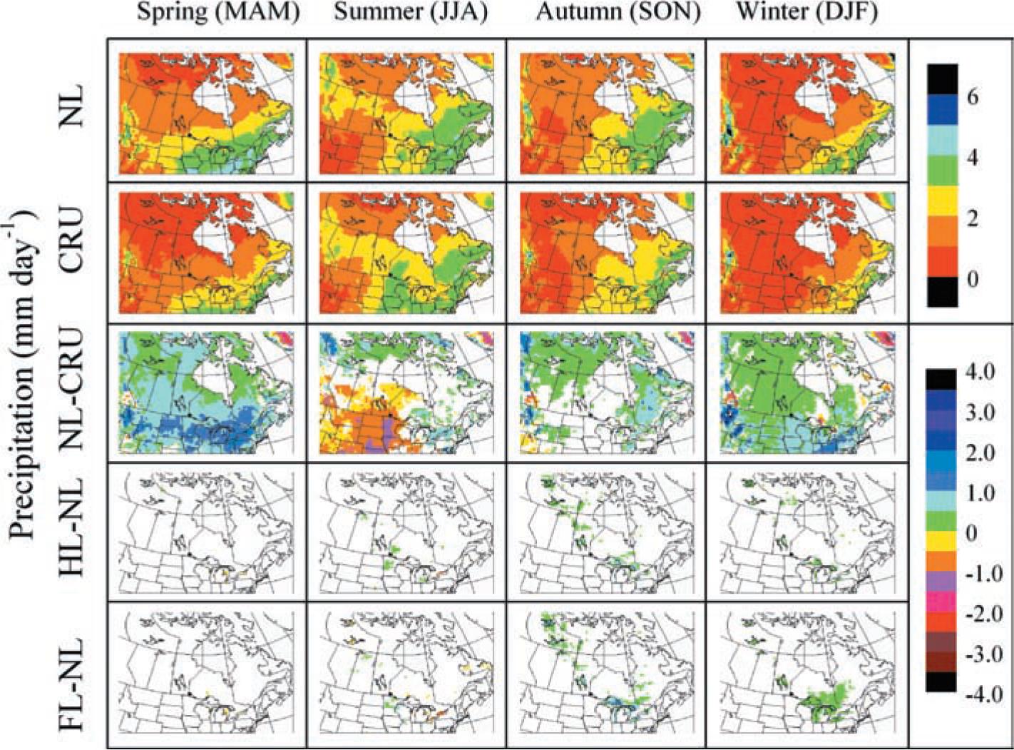
Fig. 20.
Blow up over the Great Lakes region of the precipitation differences (in mm day−1), displayed on the bottom two rows of Fig. 19.