
Table 1
Descriptive statistics. Mean and [standard deviation] for each treatment group.
| GR. 1 (SWEDES) | GR. 2 (SOMALIS) | GR. 3 (PAKISTANIS) | GR. 4 (SYRIANS) | GR. 5 (POLES) | (MIN-MAX) | |
|---|---|---|---|---|---|---|
| Warmth | 2.72 [0.66] | 1.61 [0.74] | 2.07 [0.73] | 2.04 [0.78] | 2.06 [0.69] | (0–4) |
| Competence | 2.96 [0.57] | 1.89 [0.61] | 2.47 [0.58] | 2.17 [0.65] | 2.50 [0.56] | (0–4) |
| Status | 2.19 [0.57] | 1.18 [0.55] | 1.99 [0.56] | 1.65 [0.64] | 1.68 [0.53] | (0–4) |
| Competition | 0.89 [0.71] | 1.60 [0.92] | 1.38 [0.84] | 1.47 [0.89] | 1.26 [0.76] | (0–4) |
| MCP | 2.67 [0.73] | 2.68 [0.74] | 2.70 [0.70] | 2.72 [0.74] | 2.66 [0.73] | (1–4) |
| Gender (women = 1) | 0.48 [0.50] | 0.45 [0.50] | 0.52 [0.50] | 0.49 [0.50] | 0.50 [0.50] | (1–2) |
| Age | 51.94 [16.82] | 52.36 [16.37] | 51.68 [16.52] | 51.61 [16.59] | 52.81 [16.99] | (15–87) |
| Higher education | 0.33 [0.47] | 0.32 [0.47] | 0.35 [0.48] | 0.34 [0.47] | 0.34 [0.47] | (0–1) |
| n | 596 | 557 | 519 | 575 | 552 |
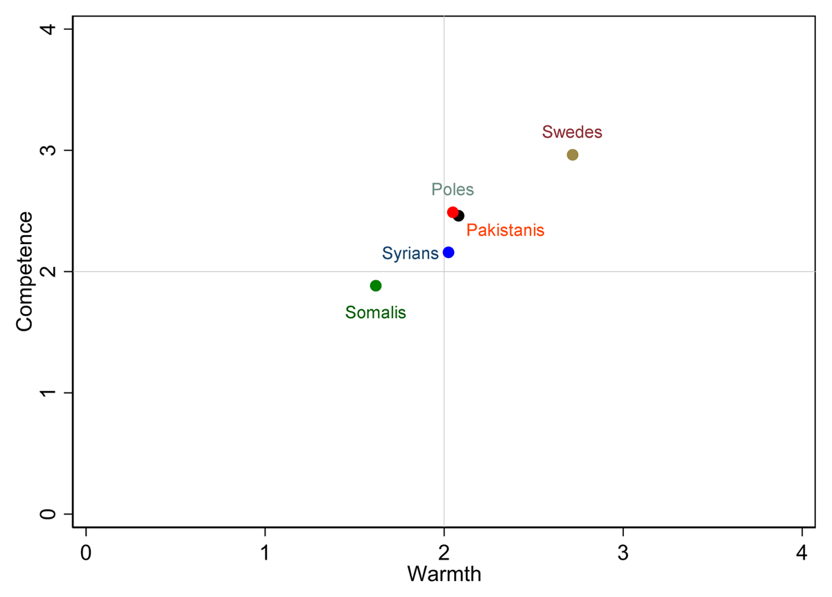
Figure 1
Placement of national groups based on competence (average of two variables) and warmth (average of two variables). N = 519–596 per group, randomly distributed.
Table 2
The relationship between stereotypes and MCP; OLS regression (n = 2799).
| WARMTH | COMPETENCE | STATUS | COMPETITION | |||||||||
|---|---|---|---|---|---|---|---|---|---|---|---|---|
| (MODEL 1) | (MODEL 2) | (MODEL 3) | (MODEL 1) | (MODEL 2) | (MODEL 3) | (MODEL 1) | (MODEL 2) | (MODEL 3) | (MODEL 1) | (MODEL 2) | (MODEL 3) | |
| Swedes (ref) | ||||||||||||
| Somalis | –1.11*** | –1.11*** | –2.03*** | –1.07*** | –1.07*** | –1.42*** | –1.02*** | –1.02*** | –1.50*** | 0.72*** | 0.73*** | 1.71*** |
| Pakistanis | –0.66*** | –0.66*** | –1.39*** | –0.50*** | –0.50*** | –0.68*** | –0.21*** | –0.21*** | –0.59*** | 0.50*** | 0.50*** | 1.24*** |
| Syrians | –0.69*** | –0.69*** | –1.44*** | –0.80*** | –0.80*** | –1.08*** | –0.54*** | –0.54*** | –1.16*** | 0.60*** | 0.60*** | 1.37*** |
| Poles | –0.65*** | –0.65*** | –0.85*** | –0.46*** | –0.46*** | –0.42*** | –0.51*** | –0.51*** | –0.58*** | 0.37*** | 0.37*** | 0.82*** |
| MCP | 0.26*** | 0.26*** | 0.07† | 0.12*** | 0.11*** | 0.05 | 0.07*** | 0.08*** | –0.03 | –0.27*** | –0.29*** | –0.07 |
| MCP*Swedes (ref) | ||||||||||||
| MCP*Somalis | 0.35*** | 0.13** | 0.18*** | –0.37*** | ||||||||
| MCP*Pakistanis | 0.27*** | 0.07 | 0.15** | –0.27*** | ||||||||
| MCP*Syrians | 0.28*** | 0.10* | 0.23*** | –0.29*** | ||||||||
| MCP*Poles | 0.07 | –0.02 | 0.02 | –0.17** | ||||||||
| Gender | 0.05† | 0.04† | 0.10*** | 0.10 | –0.01 | –0.01 | –0.00 | 0.00 | ||||
| Age | 0.00† | 0.00† | –0.00 | –0.00 | 0.00*** | 0.00*** | –0.01*** | –0.01*** | ||||
| Education | 0.05 | 0.04 | –0.05* | –0.05 | –0.05* | –0.05* | –0.18*** | –0.18*** | ||||
| cons | 2.02 | 1.92 | 2.43 | 2.64 | 2.69 | 2.85 | 2.00 | 1.86 | 2.17 | 1.62 | 2.06 | 1.48 |
| r2 | 0.25 | 0.26 | 0.27 | 0.29 | 0.29 | 0.30 | 0.27 | 0.28 | 0.29 | 0.14 | 0.16 | 0.17 |
[i] Entries are unstandardized coefficients from OLS regression models. ***p < 0.001, **p < 0.01, *p < 0.05, †p < 0.1.
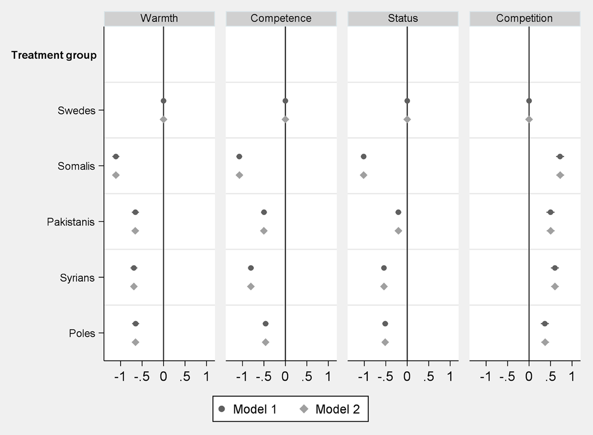
Figure 2
Effect of treatment group on stereotypes. Results from regression models 1 and 2.
Horizontal lines indicate 95% confidence intervals. Control variables: Model 1: Motivation to control prejudice. Model 2: Motivation to control prejudice, gender, age, education.
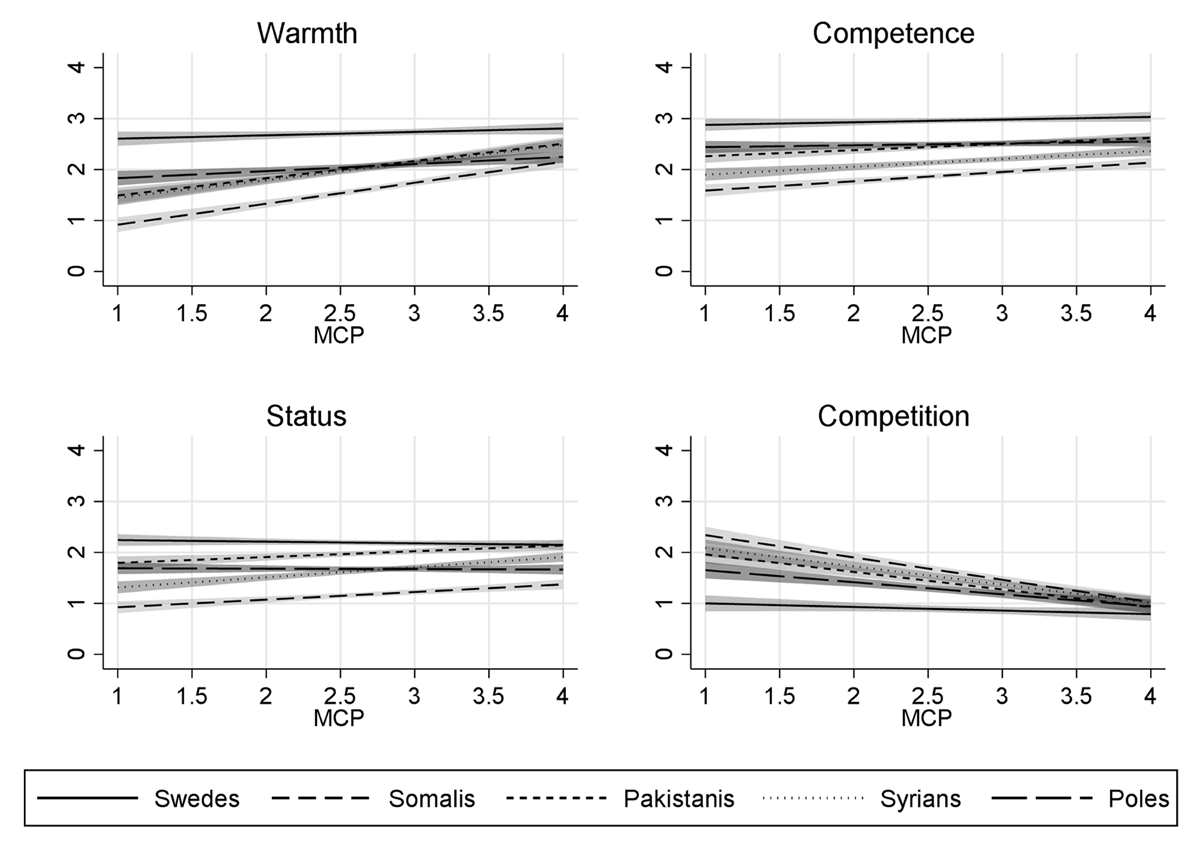
Figure 3
The interaction effects between treatment group and MCP on stereotypes. Results from regression model 3.
Shaded areas indicate 95% confidence intervals. Control variables: Model 3: Gender, age, education.