
Figure 1.
Figure 2.
Figure 3.
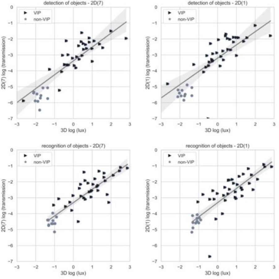
Figure 4.
Figure 5.
Figure 6.
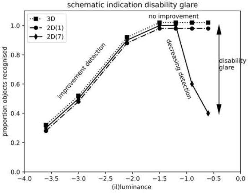
Data represent the number of objects that are detected or recognized more (second and third column) or less (fourth and fifth column) by a tenfold increase in illumination_
| Increasing slope | Decreasing slope | |||
|---|---|---|---|---|
| VIP | Non-VIP | VIP | Non-VIP | |
| 3D – detection | 0.25 log−1 (0.12) | 0.32 log−1 (0.06) | −0.03 (0.12) | 0 (0) |
| 3D – recogn | 0.29 log−1 (0.13) | 0.32 log−1 (0.06) | −0.02 (0.09) | 0 (0) |
| 2D(1) – detection | 0.28 log−1 (0.12) | 0.22 log−1 (0.05) | −0.08 (0.12) | −0.03 (0.06) |
| 2D(1) – recogn | 0.28 log−1 (0.12) | 0.28 log−1 (0.04) | −0.04 (0.14) | −0.03 (0.06) |
| 2D(7) – detection | 0.26 log−1 (0.14) | 0.22 log−1 (0.05) | −0.09 (0.14) | −0.06 (0.14) |
| 2D(7) - recogn | 0.25 log−1 (0.11) | 0.30 log−1 (0.08) | −0.11 (0.15) | −0.03 (0.10) |
Linear regression models for the four fits of figure 3_ Column R2 gives the explained variance of the linear regression models_ The goodness of the fit is provided by the last column providing the F-value and the accompanying p-value_
| slope | offset | R2 | F-value (p-value) | |
|---|---|---|---|---|
| mean [2.5%–97.5%] | mean [2.5%–97.5%] | |||
| Detection 3D-2D(1) | 0.87 [0.71–1.04] | −3.4 [−3.6; −3.2] | 0.72 | 111 (> 0.001) |
| Detection 3D-2D(7) | 0.83 [0.63–1.03] | −3.2 [−3.5; −2.9] | 0.61 | 70 (> 0.001) |
| Recognition 3D-2D(1) | 0.84 [0.69–0.99] | −3.3 [−3.5; −3.1] | 0.74 | 127 (> 0.001) |
| Recognition 3D-2D(7) | 0.89 [0.71–1.07] | −3.3 [−3.5; −3.1] | 0.69 | 97 (>0.001) |
Group characteristics of the participants in the study_
| VIP (n=40) | Non-VIP (n=11) | |
|---|---|---|
| Age (years) [min.–max.] | 54 [20–80] | 60 [51–76] |
| Female | 23 | 8 |
| Ocular disease1 |
| x |
| Visual acuity | ||
| < 0,3 LogMAR (>0.5) | 15 | 11 |
| 0.3–0.5 logMAR (0.3–0.5) | 7 | |
| 0.3–1 logMAR (0.1–0.3) | 13 | |
| >1 logMAR (<0.1) | 5 | |
| Contrast sensitivity | ||
| >1.6 logCS (normal) | 3 | 11 |
| >1.2 logCS (near normal) | 12 | |
| >0.8 logCS (moderate) | 9 | |
| >0.8 logCS (severely reduced) | ||
| unknown | ||
| 1. 6 | ||
| 10 | ||
| Reason for rehabilitation | ||
| Need for light | 17 | 0 |
| glare | 8 | 0 |
| both | 15 | 0 |
The conditions provided in the Lightlabs used during the study_ For the 2D Lightlab attenuation levels are given instead of the illumination level_
| 3D loc - 1 | 3D loc -2 | 3D loc 3 | 3D loc 4 | 2D | |
|---|---|---|---|---|---|
| Nr participants | 5 (11 non VIP) | 30 | 5 | 1 | 51 (11 non VIP) |
| Nr objects | 24 | 45 | 34 | 45 | 20 |
| Illumination levels (linear) | 1.5, 5, 15, 50, 100, 200, 500, 1000, 2000 lux | 1, 3, 5, 15, 50, 150, 500, 1000, 2000 lux | 1.5, 5, 15, 50, 100, 200, 500, 1000, 2000 lux | 5, 15, 50, 100, 200, 500, 1000, 2000 lux | 0,00025, 0.0001, 0.0078, 0.031, 0.063, 0.125, 0.25 E (attenuation) |
| Illumination levels (logarithmic) | 0.2, 0.7, 1.2, 1.7, 2.0, 2.3, 2.7, 3.0, 3.3 log(lux) | 0.0, 0.5, 0.7, 1.2, 1.7, 2.2, 2.7, 3.0, 3.3 log(lux) | 0.2, 0.7, 1.2, 1.7, 2.0, 2.3, 2.7, 3.0, 3.3 log(lux) | 0.7, 1.2, 1.7, 2.0, 2.3, 2.7, 3.0, 3.3 log(lux) | −3.6, −3.0, −2.1, −1.5, −1.2, −0.9, −0.6 logE |
| Colour temperature (K) | 3000 K | 2700 K | 3000 K | 2700 K | n.a. |