
1. INTRODUCTION
In aircraft power plant design, changes in aircraft performance requirements or flight conditions often make it necessary to find ways of increasing engine thrust. This problem is particularly pressing for the small turbojets used in Unmanned Aerial Vehicles (UAVs), since the same engine model may be selected for a variety of platforms operating in significantly different environments. Such small-scale turbojets typically share a similar architecture: a static thrust below 1000 N at sea level, a single-stage centrifugal or diagonal compressor with a low overall pressure ratio (up to 4–5), and an uncooled turbine with a turbine inlet temperature limited to about 1000°C [1]. When only a moderate thrust increase is required, a full structural redesign of the engine core is rarely economically justified. One technically simple and effective way to increase thrust without modifying the primary engine structure is the use of an ejector nozzle.
2. LITERATURE REVIEW
The first experimental tests of ejector nozzles were carried out in 1927 [2] and were aimed at demonstrating the feasibility of jet propulsion for airplanes. The first theoretical publication on ejectors is generally taken to be the paper by Keenan and Neumann [3] (1942), which presented a theoretical study of the simplest form of ejector. In the same year, Morrison [4] performed an incompressible analysis of an ejector. In 1949, von Kármán [5] set out the basic relations for cylindrical jet ejectors operating under idealized, incompressible flow conditions.
A large number of experimental and theoretical (1D and 2D) studies of ejector nozzles were carried out between 1940 and 1960; their results were summarized in 1967 in the review by K. Huang and Kisielowski [6].
One of the first studies of ejector nozzles using CFD was published in 1978 [7], in which Rushmore and Zelazny presented a 3D finite element code for analyzing ejectors (for VTOL aircraft) and mixers (for turbofans).
In recent years, a number of publications devoted to CFD studies of supersonic ejector nozzles have appeared. In 2020, Dong et al. [8] examined the ejector mode of operation of a rocket-based combined-cycle engine. In the same year, H. Huang et al. [9] investigated an integrated ejector nozzle with a tertiary door at zero flight Mach number and low nozzle pressure ratio (0.9…2.1). In 2021, H. Li et al. [10] defined and compared the over-expanded, fully expanded and under-expanded states of a steam ejector. In 2022, Z. Li and Wang [11] studied a flat ejector nozzle with a tertiary door in the full-open and open-close positions at a transonic Mach number (M = 1.2). In 2023, Z. Li et al. [12] considered the same nozzle and noted that the airflow in it exhibits lateral flow, forming a vortex ring whose size decreases gradually along the flow direction. Also in 2023, Z. Li and Wang [13] examined four versions of the tertiary air intake for the same nozzle. In 2024, Hi et al. [14] carried out a numerical simulation of an axisymmetric ejector nozzle integrated with the afterbody of an aircraft at a Mach number of 1.05.
Only a few publications are devoted to micro turbojets. In 2010, Shan et al. [15] presented experimental and CFD results for an ejector nozzle with a 12-lobed mixer for a micro turbojet engine, reporting a maximum thrust augmentation of 1.35. In 2013, Georgi and Staudacher [16] presented experimental characteristics of a micro-turbojet engine (300 N thrust) with an ejector for a scaled flight demonstrator limited to a Mach number of 0.2; the thrust augmentation achieved was no more than 4%. In 2019, Schmidt et al. [17] reported an experimental investigation of a micro-turbojet engine (180 N) with an ejector nozzle, stressing that significant thrust augmentation is possible only at take-off and low airspeed. In 2021, Schmidt and Hupfer [18] presented numerical and experimental investigations of the use of a mixer in the ejector nozzle of a micro-turbojet for UAVs, noting that the thrust augmentation of these nozzles (9.0% and 6.5%) is rather low. In 2022, Schmidt et al. [1] reported a CFD and experimental investigation of the ejector nozzle of a micro-turbojet (180 N) for a UAV, and obtained a maximum thrust augmentation of 1.11 with an 8-lobe mixer nozzle. In 2023, Cican et al. [19] studied an ejector integrated with a Jet Cat P80 micro-turbojet engine at low subsonic speeds; 3D simulations showed that the ejector increased thrust by 2…7% depending on the operating regime. In 2025, Bogoi et al. [20] presented an experimental comparative study of noise control in micro-turbojet engines with chevron and circular ejector nozzles.
A more comprehensive review was presented in [21, 22]. It follows from that review that, although ejector nozzles give a considerable thrust increase both at zero flight speed and in the supersonic range, at moderate subsonic speeds the thrust augmentation ratio φ (the ratio of ejector nozzle thrust to the thrust of the isolated primary nozzle at the same operating point) falls steeply as flight speed increases. The 1D theory of Alperin and Wu [23, 24, 25] is the only study in which a way of obtaining a substantial thrust increase within the range of moderate subsonic flight speeds has been proposed theoretically. According to this theory, which considers the mixing chamber alone under the assumption of optimal geometry of the air intake and the exhaust unit rather than a fixed-geometry ejector, two solutions exist: one corresponds to subsonic and the other to supersonic speed at the exit of the mixing chamber. Moreover, within the range of moderate subsonic flight speeds the first solution offers practically no opportunity to increase thrust, whereas the second solution looks very attractive, although its physical existence is open to doubt, which indicates that the subject has not been studied sufficiently. The goal of this work is therefore stated as an attempt to corroborate, using computational fluid dynamics, the existence of the second solution of Alperin’s 1D theory for an ejector nozzle.
3. METHODOLOGY
As mentioned above, the 1D theory of Alperin and Wu [23, 24, 25] is the only study in which a way of obtaining a substantial thrust increase within the range of moderate subsonic flight speeds has been proposed theoretically. The theory rests on the following assumptions:
1) All fluids are compressible and thermally and calorically perfect.
2) Skin friction and blockage losses are neglected.
3) Mixing is initiated in a constant area duct at the location where the primary flow is fully expanded (primary flow pressure is equal to the local secondary flow pressure).
4) Complete mixing occurs in a constant cross-sectional channel.
5) Ejector surfaces are adiabatic [23].
Alperin and Wu then consider the mixing chamber alone (assuming an isentropic air intake and exit) and, using conservation of mass flow, conservation of energy, the momentum theorem and the equations of state, obtain a quadratic equation for the Mach number at the end of the mixing chamber. Solving this equation gives two roots: one is subsonic, always exists and yields the so-called optimal solution, while the other is supersonic and can exist only when the change in total entropy due to the mixing process is positive. Removing the intervals in which the change in total entropy is negative, they obtain the so-called limit solution.
Using this 1D theory, the ideal thrust augmentation ratio of the ejector nozzle was calculated for the first and second solutions over the range of the ratio of mixing chamber area to primary nozzle exit area α* = 1...25, at a flight Mach number M∞ = 0.6. Fig. 1 shows that, for the first solution, the ideal thrust augmentation ratio over α* = 1...25 is below unity and decreases slightly, which makes the use of an ejector nozzle unreasonable. For the second solution, the ideal thrust augmentation ratio over α* = 1...25 lies in the interval [1…4] and increases as α* increases, which is encouraging.
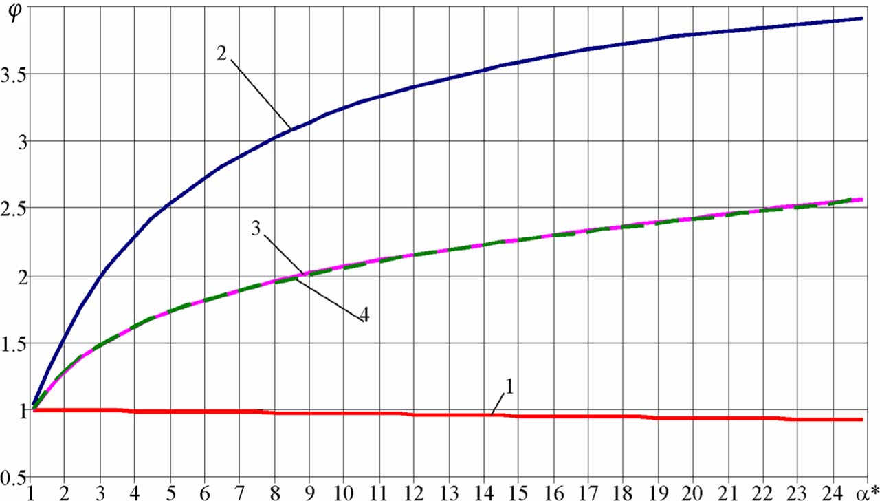
Fig.1.
Ejector nozzle thrust augmentation ratio vs. α*: 1 – first solution, ideal; 2 – second solution, ideal; 3 – second solution, with nozzle underexpansion losses from 1D theory; 4 – second solution, with nozzle underexpansion losses from 2D theory.
The nozzle underexpansion losses caused by overexpansion at the throat under the nozzle starting condition were estimated using the publication of Hermann [26]. The curves of thrust augmentation ratio for the second solution obtained with nozzle underexpansion losses from 1D and from 2D theory almost coincide with each other; with these losses taken into account, the thrust augmentation ratio for the second solution over α* = 1...25 lies within the interval [1…2.5] and increases as α* increases.
The dependence of the thrust augmentation ratio on flight Mach number was then calculated for each of the two solutions (Fig. 2; solid lines – first solution, dashed lines – second solution) using Alperin’s 1D theory [23, 24], without allowance for losses, for α* = 3, α* = 4, α* = 5 and α* = 7, with the engine parameters held “frozen”.
It should be stressed that these solutions are optimal or limiting ones (subject to the conditions of positive change in total entropy and positive Mach number at the ejector nozzle exit), so they correspond to the maximum possible value of φ as a function of the Mach number at the entrance to the mixing chamber. The values of φ for supersonic flight speeds therefore correspond to extreme points, at which a small deviation from the optimal Mach number at the entrance to the mixing chamber causes a sharp decrease; this practically rules out the use of these solutions.
Fig. 2 shows that, within the flight Mach number range [0.4…1.4], the values of the thrust augmentation ratio given by the first (subsonic) solution, without allowance for losses, do not exceed unity, which agrees with the charts of Alperin and Wu [23]. Hence, within the accuracy of Alperin’s theory, a thrust increase cannot be obtained in this range of Mach numbers using an ejector nozzle with subsonic speed at the exit of the mixing chamber.
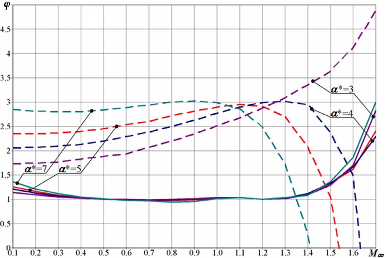
Fig. 2.
Ejector nozzle thrust augmentation ratio vs. flight Mach number (without taking into account losses).
Reducing the values of the thrust augmentation ratio given by the second (supersonic) solution by one third yields approximately the values of the thrust augmentation ratio obtained when underexpansion losses are taken into account (see Fig. 1).
4. PROBLEM STATEMENT
On the basis of the dimensions of the mixing chamber, the value α* = 5 was assumed initially for the study that follows; at M∞ = 0.6 this should provide a thrust augmentation ratio φ = 1.72 according to the second solution, with nozzle underexpansion losses taken into account.
5. MODELS AND METHODS
5.1. Physical Models
At this stage of the study, axisymmetric models were used in order to reduce computational time. Thirty-two 2D models of the computational domain (α* = 5) were built in the Kompas 19 system. So that the boundary conditions could be specified at an “infinite” distance from the nozzle, the computational domain was made large enough: about 8L (3110 mm) long in the airflow direction and about 6.75R (500 mm) in radius, where L = 388 mm is the total length of the engine and R = 74 mm is the middle radius of the engine (Fig. 3).

Fig. 3.
Computational domain (configurations 1–5).
Configurations 1–5 (α* = 5) (Fig. 4) were intended for the mesh independence study.
The features of the configurations for α* = 5 (Fig. 5) and α* = 4 (Fig. 6) are described in Section 7 (Results and Discussion).
5.2. Meshing Method
Standard ANSYS Meshing software was used for mesh generation. Five unstructured meshes with quadrilateral element sizes of 20, 15, 10, 7.5 and 5 mm were used for the mesh independence study. In addition, each mesh was refined near all the nozzle walls by setting Insert\Sizing\Element Size to 0.40, 0.30, 0.20, 0.15 and 0.10 mm respectively (see Fig. 4).
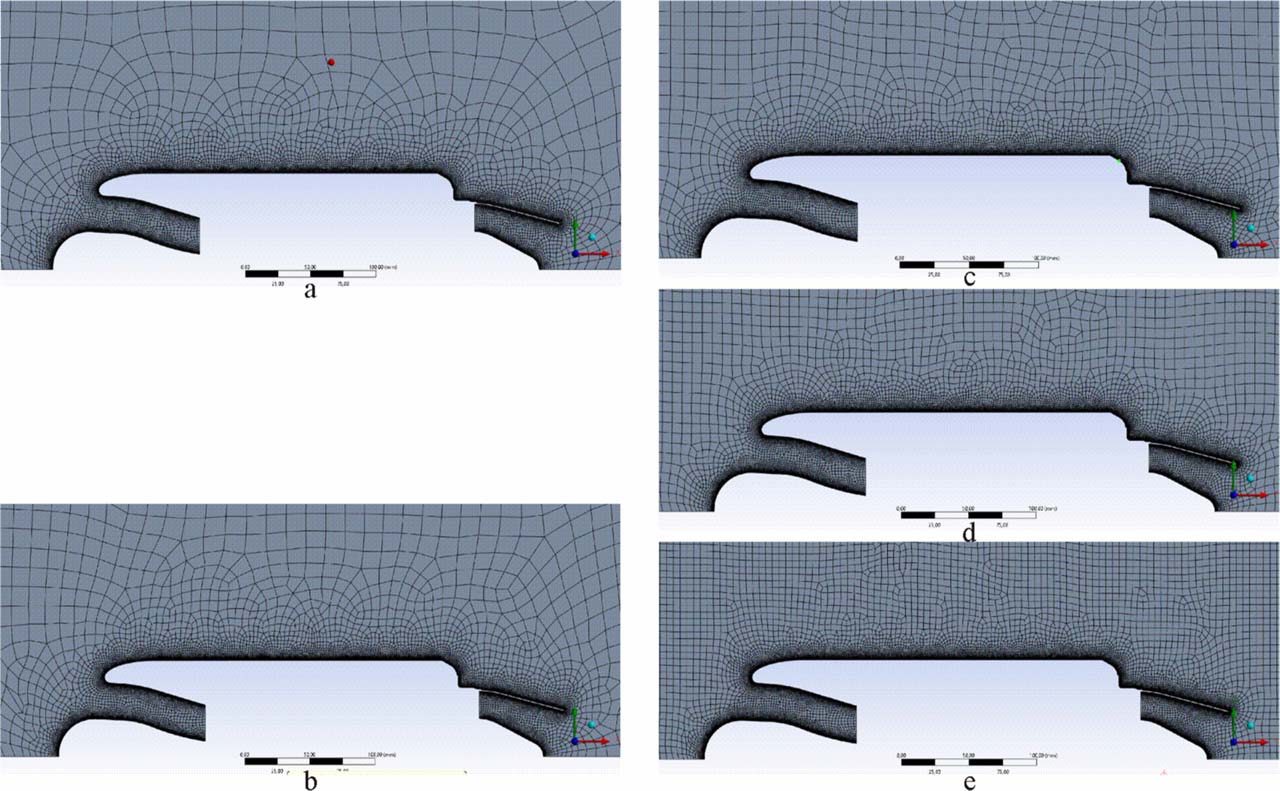
Fig. 4.
The five meshes considered: a – 20 mm; b – 15 mm; c – 10 mm; d – 7.5 mm; e – 5 mm.
5.3. Boundary Conditions and Solution Methods
Fig. 7 shows the boundary types of the model. The left and top boundaries were adopted as pressure-far-field (with M∞ = 0.6 for all configurations), and the right boundary as pressure-outlet. All the engine surfaces were set as no-slip insulating walls. The outlet to the engine compressor was adopted as the mass-flow-outlet boundary type, and the inlet of the primary flow from the gas generator into the engine nozzle as the pressure-inlet boundary type. Static pressure, static temperature, Mach number, turbulence intensity and hydraulic diameter were specified on the pressure-far-field boundaries. Static pressure, total temperature, Mach number, turbulence intensity and hydraulic diameter were specified on the pressure-outlet boundary. The air flow rate was specified on the mass-flow-outlet boundary. Total pressure, total temperature, turbulence intensity and hydraulic diameter were specified on the pressure-inlet boundary. The values of the corresponding boundary parameters are listed in Table 1.
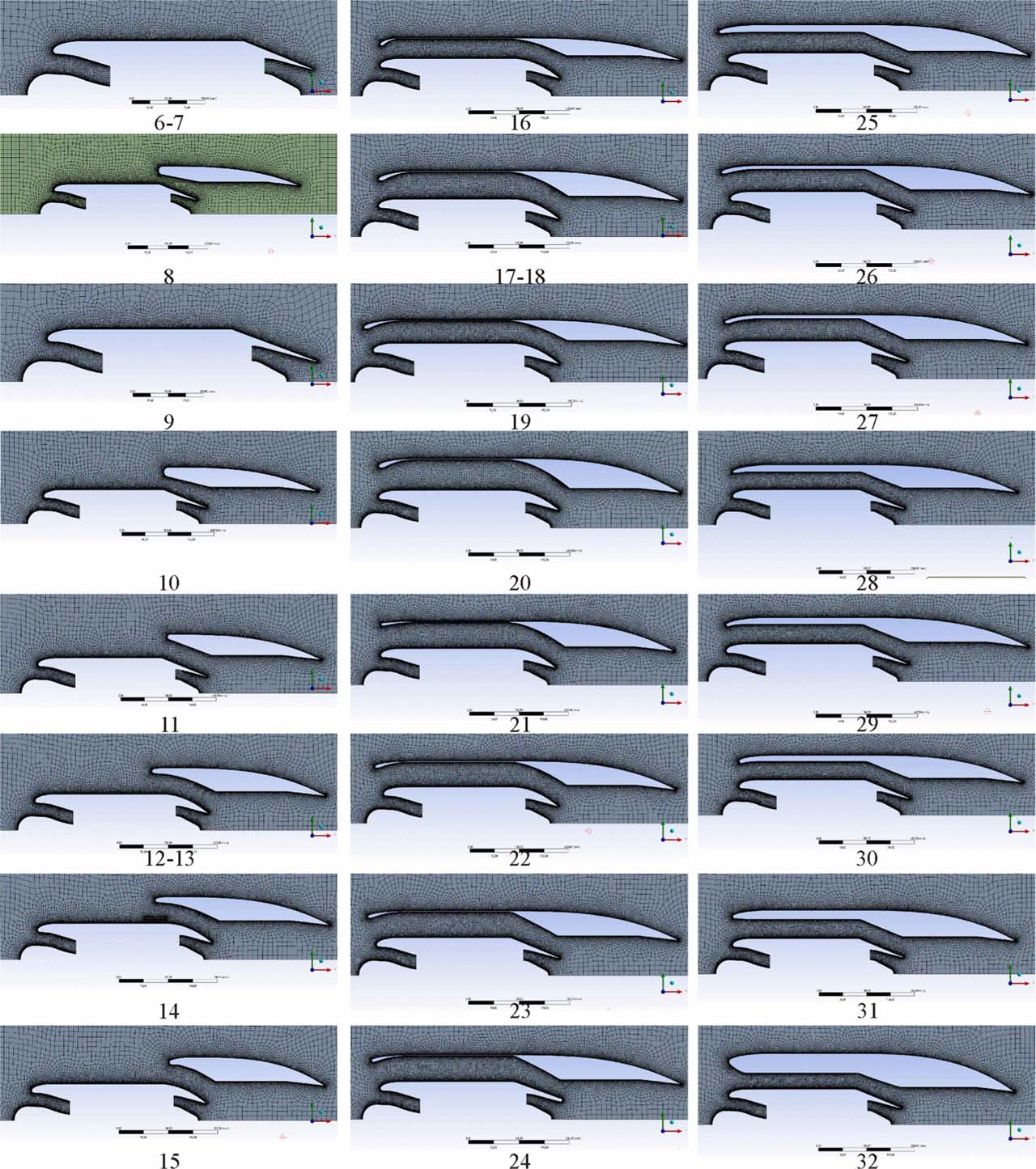
Fig. 5.
Configurations considered (α*= 5).
ANSYS Fluent 2024R1 software was used for the numerical simulation. The density-based solver was used, since attempts to use the pressure-based solver resulted in divergence in ANSYS Fluent. On the basis of study [27], the k-ω BSL turbulence model with Options\Compressibility Effects was used for all the computations. Air was used as the fluid, treated as an ideal gas whose viscosity was calculated by the three-coefficient Sutherland method. From configuration 18 onwards, the variation of the coefficient Cp with temperature was taken into account by means of a piecewise-polynomial approximation (Properties/Cp/piecewise-polynomial); configurations 1–5 were then recalculated with this variation of Cp taken into account. An implicit formulation was applied (Solution/Methods/Formulation=Implicit), together with a first-order upwind scheme for the turbulent kinetic energy and specific dissipation rate equations [28]. In addition, the residuals were set to 0.0001. Finally, hybrid initialization was used.
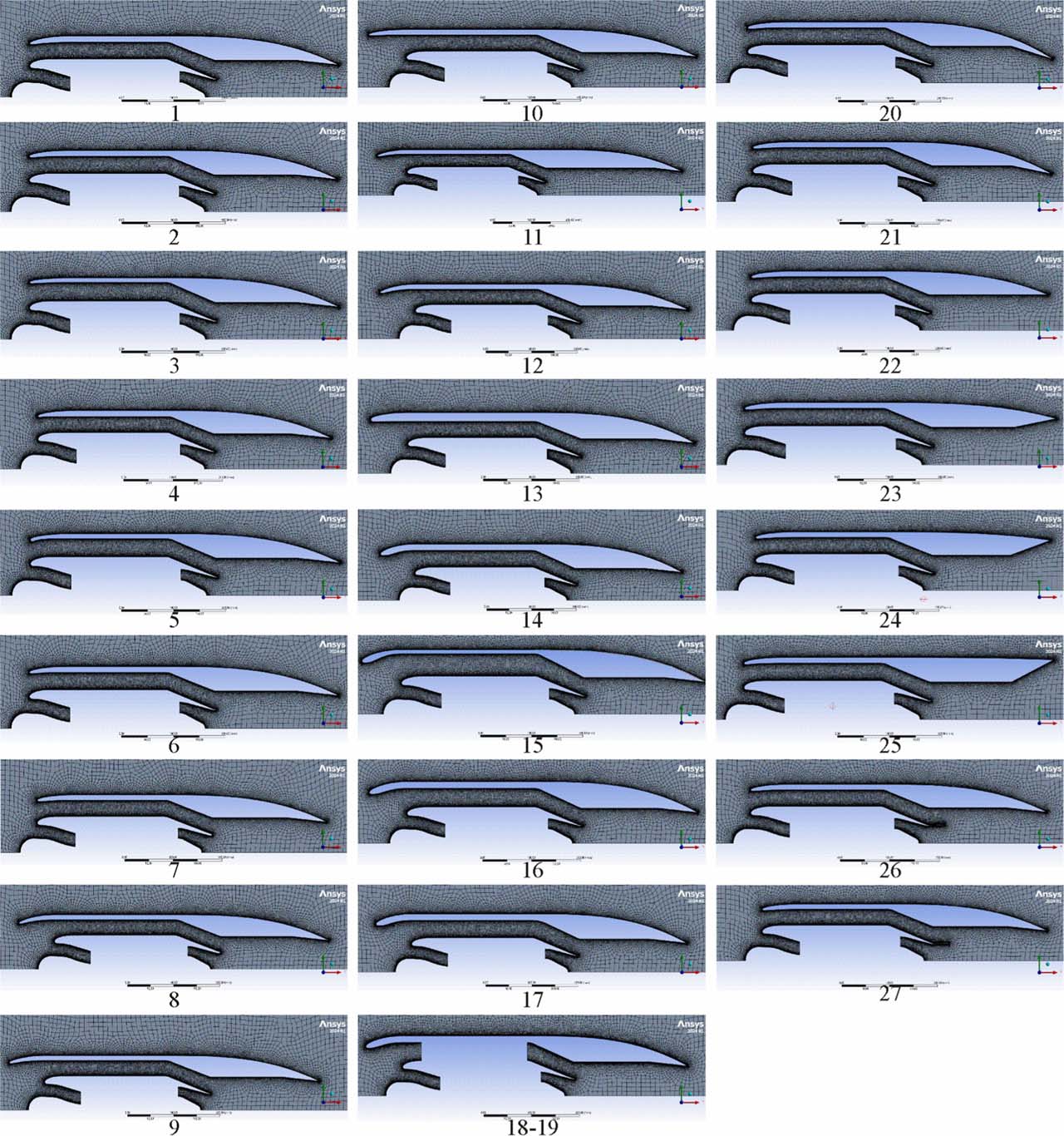
Fig. 6.
Configurations considered (α*= 4).
6. MODEL VERIFICATION AND VALIDATION
6.1. Estimation of Uncertainty Due to Discretization
A long-established procedure for estimating the discretization error using the Grid Convergence Index (GCI) was proposed in [29], and the procedure was set out in detail in [30]. It is this procedure that is used below.
As mentioned above, five meshes with element sizes of 20, 15, 10, 7.5 and 5 mm were generated in order to verify mesh independence; they are denoted by the indices 1–5 respectively.
The integral parameter (thrust) and the representative mesh cell size obtained from the computations on the five meshes considered are shown in Table 2. A comparative estimation of the computational results on meshes 1–2–3, 2–3–4 and 3–4–5, based on the methodology of [29, 30], is presented in Table 3.
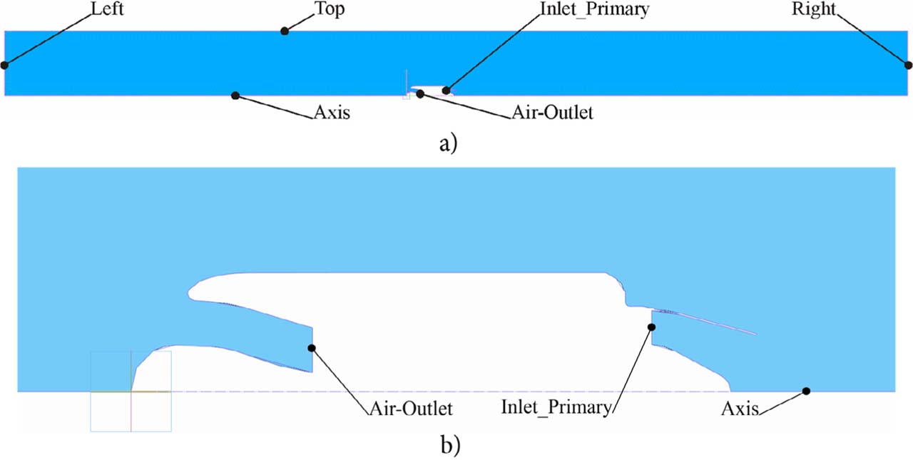
Fig. 7.
Model boundaries.
Also, taking into account the difficulties in reaching convergence on meshes 4 and 5, it is reasonable to adopt mesh 3 (10 × 0.20 mm) for the computations that follow.
6.2. Comparison of the calculated integral parameters on different meshes with the results of the 1D computation
The following engine integral parameters were used for the comparison: gas flow rate; average speed within the exit cross-section; average static pressure within the exit cross-section; nozzle thrust; and engine thrust. The corresponding differences (Δm – for flow rate, Δv – for speed, Δp – for pressure, ΔNozzle Th – for nozzle thrust, ΔTh – for engine thrust) are shown in Table 4:
where PFluent is the value of the parameter from the 2D computation in ANSYS Fluent, and P1D is the value of the same parameter from the 1D calculation made by the engine developer using a component-based thermodynamic model.Table 1.
Values of corresponding boundary parameters.
| Boundary/Parameter | Total/static pressure, Pa | Turbulence intensity, % | Mach number | Flow rate, kg/s | Total/static temperature, K |
|---|---|---|---|---|---|
| Left (Pressure-far-field) | –/101325 | 1.0 | 0.6 | – | –/288.15 |
| Top (Pressure-far-field) | –/101325 | 1.0 | 0.6 | – | –/288.15 |
| Right (Pressure outlet) | –/101325 | 1.0 | – | – | 308.89/– |
| AirOutlet (Mass-flow-outlet) | – | – | – | 0.99 | – |
| InletPrimary (Pressure-inlet) | 209787/– | 10.0 | – | – | 993.05/– |
Table 2.
Parameter values on the corresponding meshes.
| Mesh, | Integral parameter, N | Representative mesh cell size, m |
|---|---|---|
| 1 (20 × 0.40 mm) | 395.65 | 1.24×10⁻² |
| 2 (15 × 0.30 mm) | 396.21 | 1.01×10⁻² |
| 3 (10 × 0.20 mm) | 396.31 | 7.46×10⁻³ |
| 4 (7.5 × 0.15 mm) | 394.66 | 5.94×10⁻³ |
| 5 (5 × 0.10 mm) | 395.60 | 4.23×10⁻³ |
Table 3.
Comparative estimation of the computational results.
| Parameter | Meshes 1–2–3 | Meshes 2–3–4 | Meshes 3–4–5 |
|---|---|---|---|
| h1, m | 7.46×10⁻³ | 5.94×10⁻³ | 4.23×10⁻³ |
| h2, m | 1.01×10⁻² | 7.46×10⁻³ | 5.94×10⁻³ |
| h3, m | 1.24×10⁻² | 1.01×10⁻² | 7.46×10⁻³ |
| P1, N | 396.31 | 394.66 | 395.60 |
| P2, N | 396.21 | 396.31 | 394.66 |
| P3, N | 395.65 | 396.21 | 396.31 |
| r32 | 1.229 | 1.350 | 1.255 |
| r21 | 1.350 | 1.255 | 1.403 |
| s | 1 | −1 | −1 |
| p | 8.525 | 17.788 | 2.119 |
| CR | 0.192 | −15.573 | −0.568 |
| [0; 1) – monotonic convergence | (−∞; −1) – oscillating divergence | [−1; 0) – oscillating convergence | |
| fex, N | 396.32 | 394.63 | 396.49 |
| e32, % | 0.140 | 0.027 | 0.419 |
| e21, % | 0.027 | 0.419 | 0.238 |
| GCI32, % | 0.036 | 0.000 | 0.848 |
| GCI21, % | 0.003 | 0.009 | 0.283 |
| < 1% – for detailed calculations | < 1% – for detailed calculations | < 1% – for detailed calculations | |
| AR | 1.000 | 0.0003 | 1.463 |
| [0.95; 1.05] – optimum | (−∞; 0.95) – mesh should be improved | (1.05; ∞) – mesh should be improved | |
| hreq | 3.74×10⁻³ | 4.57×10⁻³ | 2.33×10⁻⁶ |
Table 4 shows that, for all the meshes, the differences do not exceed 4.7% for flow rate, 17.6% for speed, 25.8% for pressure, 2.7% for nozzle thrust and 3.8% for engine thrust. It is also clear that, except for the engine thrust, the lowest differences occur on mesh 3 (10 × 0.20 mm), which was the mesh adopted for further use.
Table 4.
Differences of integral parameter calculations.
| Parameter | Mesh 20 mm | Mesh 15 mm | Mesh 10 mm | Mesh 7.5 mm | Mesh 5 mm |
|---|---|---|---|---|---|
| Δm, % | −4.438 | −4.173 | −4.076 | −4.605 | −4.329 |
| Δv, % | −17.564 | −16.510 | −16.232 | −17.036 | −16.542 |
| Δp, % | 25.717 | 24.289 | 23.876 | 24.894 | 24.288 |
| ΔNozzle Th, % | −2.668 | −2.488 | −2.442 | −2.888 | −2.640 |
| ΔTh, % | −3.494 | −3.259 | −3.333 | −3.737 | −3.507 |
The large differences in speed and static pressure in the exit cross-section can be explained by the nonlinearity of the sonic line, which is reproduced in ANSYS Fluent but is neglected in the 1D theory.
7. RESULTS AND DISCUSSION
Once the computation of each configuration was complete, the following were obtained:
fields of static temperature, which were plotted for some configurations (Fig. 13). The static temperature distribution describes indirectly the mixing of the primary flow with the secondary flow. As can be seen, mixing proceeds too slowly, and the flows do not have enough time to mix before leaving the mixing chamber. This proves that a mixer needs to be installed;
charts of the Mach number distribution over representative nozzle cross-sections;
charts of the static pressure distribution over representative nozzle cross-sections;
nozzle integral parameters (Table 5).
7.1. Configurations for α* = 5
Configurations 1–5 (see Fig. 4) represent the basic engine and were used for the mesh independence study. On the basis of these calculations, the mesh with a cell size of 10 mm was selected (see Section 6). This study also drew attention to the flow separation zone at the aft end of the engine, as a result of which some fairings were added.
Configurations 6, 7 and 9 (see Fig. 5) represent the basic engine with various fairings. As an example, Fig. 8 shows the pathline patterns for configurations 3 and 6. An air separation zone can be seen at the end of the engine without a fairing (Fig. 8, a), and a substantially smaller separation zone for the engine with a fairing (Fig. 8, b).
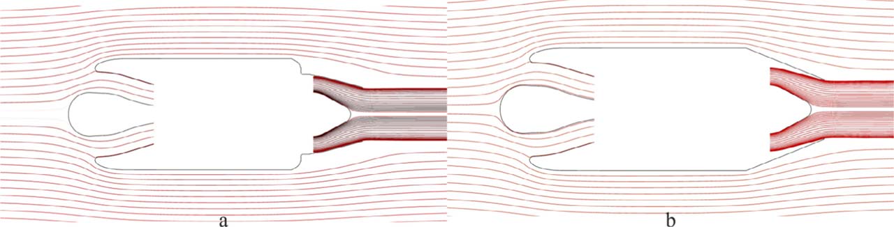
Fig. 8.
Pathline patterns for configurations 3 and 6 (α* = 5).
From configuration 8 onwards (except in specially stated cases), the engine with a fairing was equipped with an ejector nozzle consisting of a mixing chamber of constant cross-sectional area (corresponding to the specified α*) and a convergent exhaust unit, in which the supersonic flow leaving the mixing chamber should decelerate so as to raise the static pressure to atmospheric. The exit area of the exhaust unit was calculated from the starting condition, following Alperin and Wu [24], thereby setting the design system of shocks within the exhaust unit.
Configurations 8 and 10–15 were used to work through the shape of the aft air intake. Since we failed to reach the secondary flow rate specified by Alperin’s model, and since the second solution does not exist for values of the Mach number at the entrance to the mixing chamber below the design point, we were forced to look for another shape of air intake.
Configurations 16–18 and 20–21 were used to work through the shape of a nose air intake whose entry plane coincides with the entry plane of the engine air intake. Since we again failed to reach the secondary flow rate specified by Alperin’s model, we were forced to shift the air intake further forward in configuration 19.
Configurations 19 and 22–26 were used to work through the shape of a nose air intake whose entry plane is shifted forward relative to the entry plane of the engine air intake by half the length of the central body. Flow separation zones were almost absent. Since we still failed to reach the secondary flow rate specified by Alperin’s model, it was considered reasonable to return the entry plane of the air intake to the engine entry plane, but this time without any constraint between the radius of the external shell and the radius of the duct.
Configurations 27–32 were used to make further attempts to reach the secondary flow rate specified by Alperin’s model, by reshaping the air intake with a specified area distribution (perpendicular to the axis) and by varying the duct area. Once again, however, we failed to reach the specified secondary flow rate for α* = 5. Since the calculated secondary flow rate was close to the value specified for α* = 4, it was considered reasonable to move to α* = 4, which at M∞ = 0.6 should provide a thrust augmentation ratio φ = 1.62 according to the second solution, with nozzle underexpansion losses taken into account.
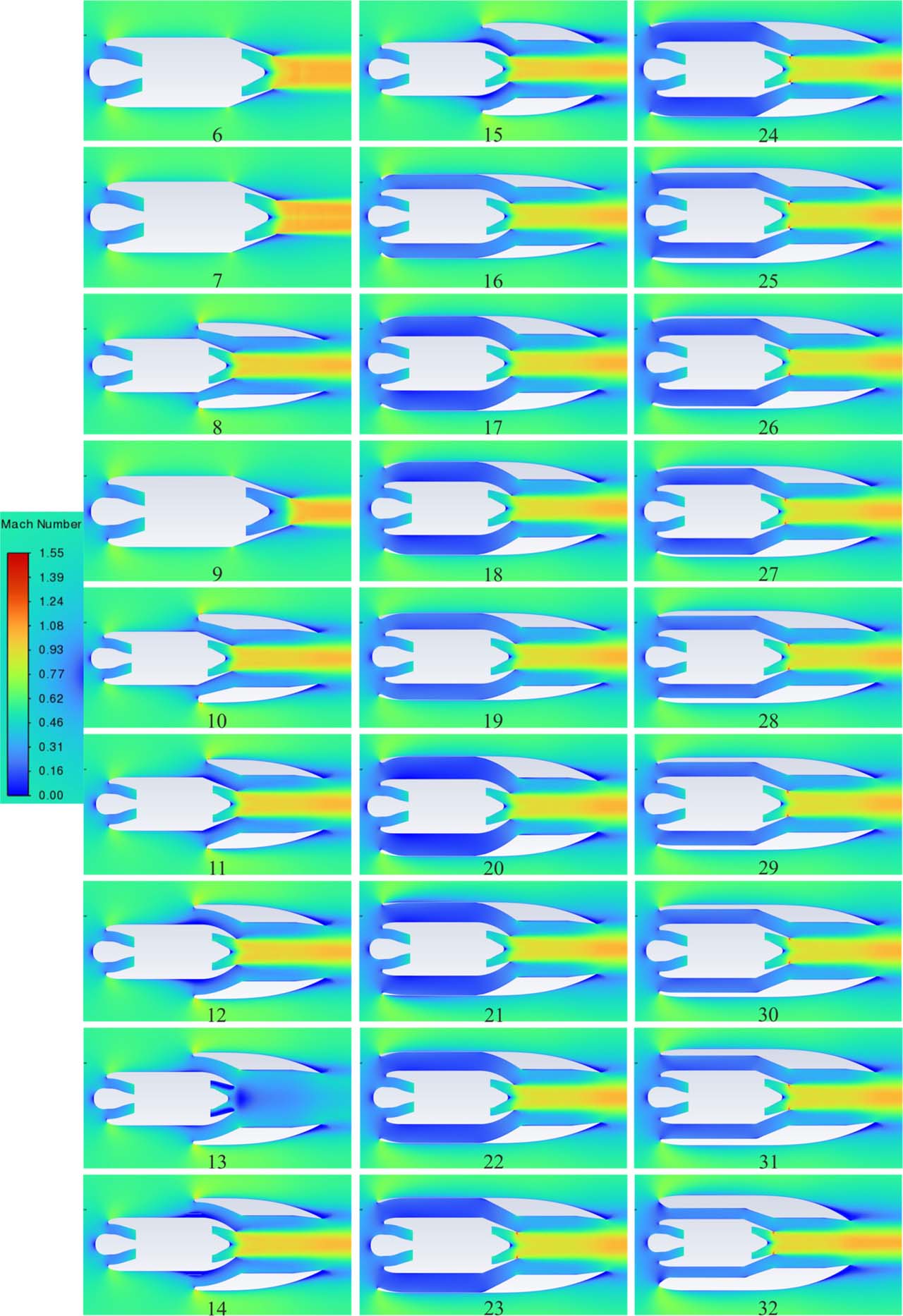
Fig. 9.
Fields of Mach number for the configurations considered (α* = 5).
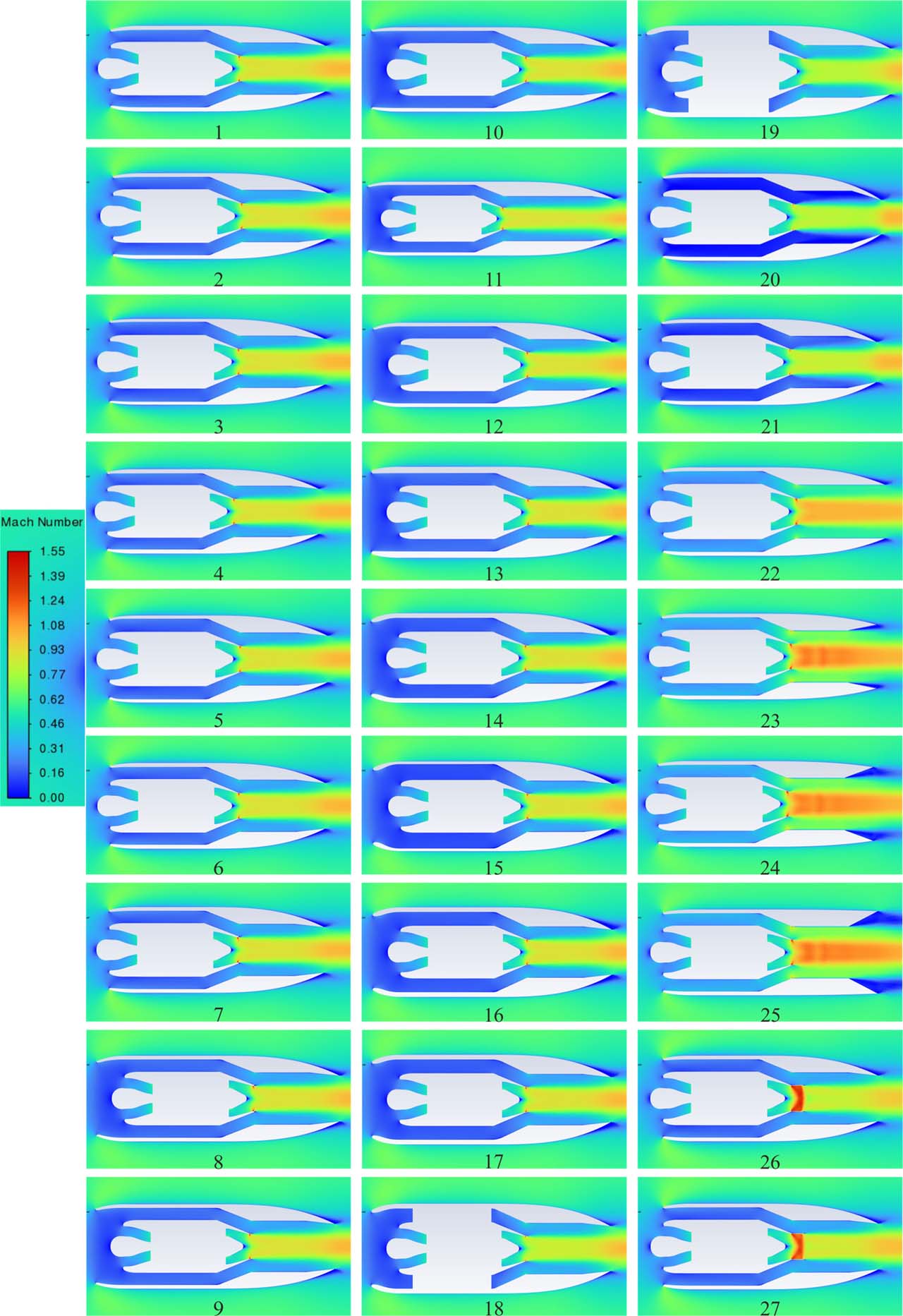
Fig. 10.
Fields of Mach number for the configurations considered (α* = 4).
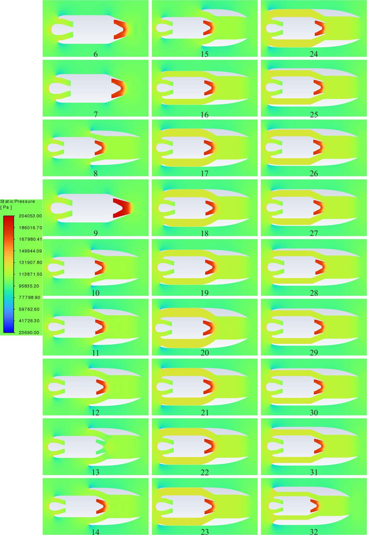
Fig. 11.
Fields of static pressure for the configurations considered (α* = 5).
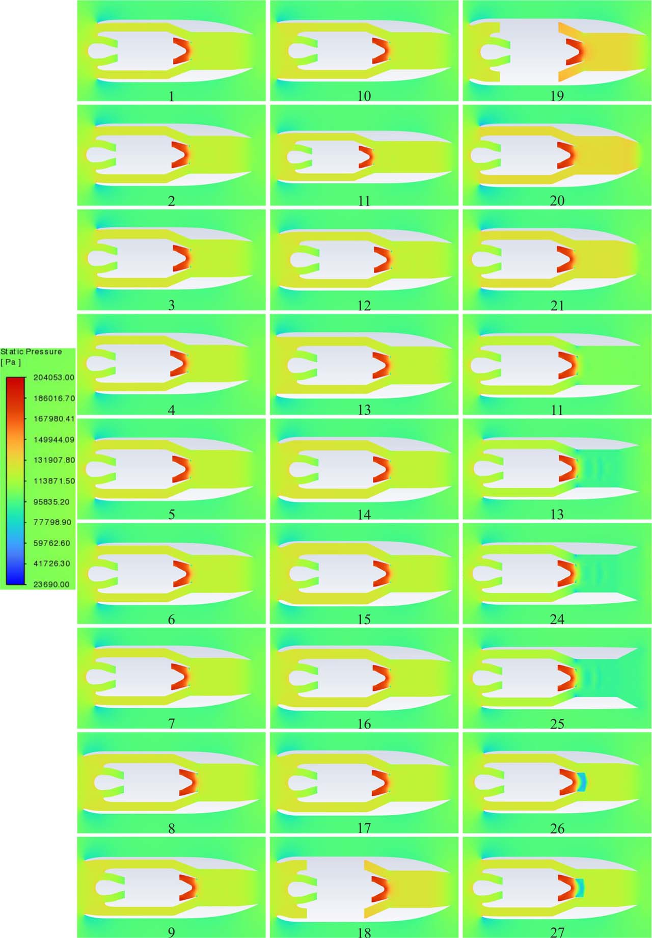
Fig. 12.
Fields of static pressure for the configurations considered (α* = 4).
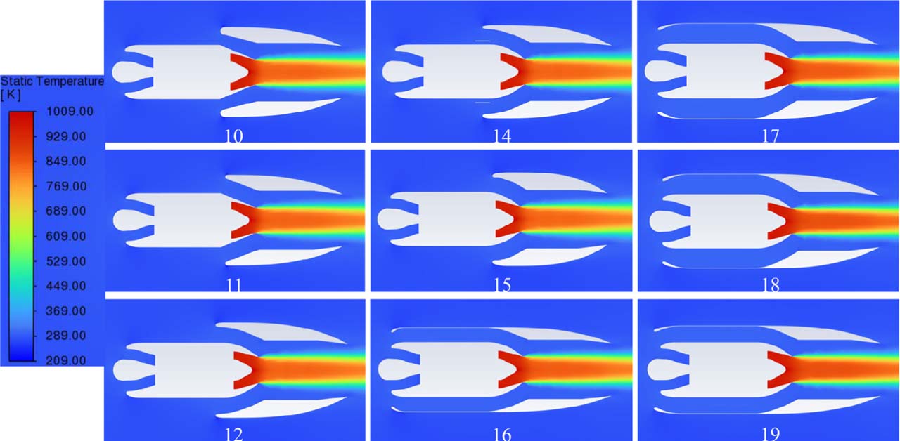
Fig. 13.
Fields of static temperature for some of the configurations considered (α* = 5).
Table 5.
Results of integral parameter calculations.
| Parameter/Configuration | Secondary flow Mach number at the entrance of mixing chamber | Primary flow rate, kg/s | Entrainment ratio | Thrust, N | Augmentation ratio, φ |
|---|---|---|---|---|---|
| Alperin | 0.4119 | — | 2.868 | — | 1.72 |
| Base engine | — | 1.0102 | — | 409.978 | — |
| 1 (α* = 5) | — | 0.96537 | — | 395.65 | — |
| 2 (α* = 5) | — | 0.96804 | — | 396.21 | — |
| 3 (α* = 5) | — | 0.96903 | — | 396.31 | — |
| 4 (α* = 5) | — | 0.96368 | — | 394.66 | — |
| 5 (α* = 5) | — | 0.96647 | — | 395.60 | — |
| 6 (α* = 5) | — | 0.97104 | — | 394.35 | — |
| 7 (α* = 5) | — | 0.97484 | — | 395.92 | — |
| 8 (α* = 5) | 0.32082 | 0.96839 | 2.31028 | 299.26 | 0.72994 |
| 9 (α* = 5) | — | 0.61498 | — | 251.28 | — |
| 10 (α* = 5) | 0.32750 | 0.97310 | 2.33550 | 301.40 | 0.73516 |
| 11 (α* = 5) | 0.34470 | 0.96667 | 2.42548 | 305.87 | 0.74607 |
| 12 (α* = 5) | 0.33997 | 0.96408 | 2.41586 | 305.31 | 0.74470 |
| 13 (α* = 5) | 0.46743 | 0.23817 | 13.57310 | 227.01 | 0.55370 |
| 14 (α* = 5) | 0.34294 | 0.96564 | 2.40173 | 304.53 | 0.74279 |
| 15 (α* = 5) | 0.35425 | 0.96738 | 2.42944 | 298.82 | 0.72887 |
| 16 (α* = 5) | 0.34583 | 0.94622 | 2.83003 | 365.90 | 0.89247 |
| 17 (α* = 5) | 0.34722 | 0.94040 | 2.97538 | 382.91 | 0.93398 |
| 18 (α* = 5) | 0.34472 | 0.93197 | 2.98313 | 383.83 | 0.93622 |
| 19 (α* = 5) | 0.35423 | 0.93440 | 2.95817 | 385.23 | 0.93964 |
| 20 (α* = 5) | 0.31634 | 0.92613 | 2.84300 | 381.47 | 0.93047 |
| 21 (α* = 5) | 0.33955 | 0.93160 | 2.83899 | 386.71 | 0.94323 |
| 22 (α* = 5) | 0.34451 | 0.92628 | 2.85432 | 386.43 | 0.94256 |
| 23 (α* = 5) | 0.37377 | 0.97795 | 2.66855 | 407.85 | 0.99482 |
| 24 (α* = 5) | 0.40219 | 0.98181 | 2.62750 | 405.87 | 0.98997 |
| 25 (α* = 5) | 0.39948 | 0.98102 | 2.61869 | 401.61 | 0.97958 |
| 26 (α* = 5) | 0.37102 | 0.97963 | 2.64032 | 410.45 | 1.00115 |
| 27 (α* = 5) | 0.37075 | 0.98006 | 2.62426 | 404.57 | 0.98681 |
| 28 (α* = 5) | 0.36716 | 0.98029 | 2.60928 | 402.62 | 0.98206 |
| 29 (α* = 5) | 0.37423 | 0.97742 | 2.60485 | 406.13 | 0.99062 |
| 30 (α* = 5) | 0.36818 | 0.97993 | 2.61096 | 402.31 | 0.98130 |
| 31 (α* = 5) | 0.36976 | 0.98077 | 2.61755 | 403.16 | 0.98337 |
| 32 (α* = 5) | 0.36390 | 0.97955 | 2.54888 | 378.82 | 0.92399 |
| Alperin | 0.379 | — | 2.008 | — | 1.62 |
| Base engine | — | 1.0102 | — | 409.978 | — |
| 1 (α* = 4) | 0.35692 | 0.97862 | 2.04513 | 402.43 | 0.98158 |
| 2 (α* = 4) | 0.35962 | 0.97930 | 2.05995 | 398.65 | 0.97238 |
| 3 (α* = 4) | 0.35893 | 0.97805 | 2.06253 | 399.83 | 0.97525 |
| 4 (α* = 4) | 0.35652 | 0.97793 | 2.04692 | 404.07 | 0.98559 |
| 5 (α* = 4) | 0.35750 | 0.97854 | 2.04527 | 397.83 | 0.97036 |
| 6 (α* = 4) | 0.35814 | 0.97848 | 2.05250 | 399.17 | 0.97363 |
| 7 (α* = 4) | 0.36632 | 0.97972 | 2.03578 | 405.58 | 0.98928 |
| 8 (α* = 4) | 0.36516 | 0.97918 | 2.04474 | 406.69 | 0.99198 |
| 9 (α* = 4) | 0.35050 | 0.97629 | 2.06375 | 400.55 | 0.97699 |
| 10 (α* = 4) | 0.35007 | 0.97877 | 2.05843 | 400.61 | 0.97715 |
| 11 (α* = 4) | 0.34451 | 0.97490 | 2.03757 | 402.30 | 0.98127 |
| 12 (α* = 4) | 0.35006 | 0.97648 | 2.06037 | 403.69 | 0.98467 |
| 13 (α* = 4) | 0.35034 | 0.98014 | 2.04143 | 402.45 | 0.98165 |
| 14 (α* = 4) | 0.35651 | 0.97861 | 2.04413 | 398.08 | 0.97097 |
| 15 (α* = 4) | 0.35597 | 0.98016 | 2.03369 | 395.00 | 0.96346 |
| 16 (α* = 4) | 0.35525 | 0.97989 | 2.04758 | 396.51 | 0.96716 |
| 17 (α* = 4) | 0.33691 | 0.97977 | 2.04349 | 395.18 | 0.96389 |
| 18 (α* = 4) | 0.38328 | 0.96484 | 2.33288 | 464.50 | 1.13298 |
| 19 (α* = 4) | 0.40915 | 0.94874 | 2.63502 | 512.45 | 1.24994 |
| 20 (α* = 4) | 0.09572 | 0.96209 | 0.61172 | 375.47 | 0.91584 |
| 21 (α* = 4) | 0.22171 | 0.96876 | 1.35933 | 400.38 | 0.97658 |
| 22 (α* = 4) | 0.58058 | 0.98028 | 2.89229 | 385.55 | 0.94040 |
| 23 (α* = 4) | 0.71614 | 0.98227 | 3.14938 | 315.27 | 0.76900 |
| 24 (α* = 4) | 0.70802 | 0.97691 | 3.19422 | 167.34 | 0.40818 |
| 25 (α* = 4) | 0.73642 | 0.98236 | 3.17467 | 13.62 | 0.03323 |
| 26 (α* = 4) | 0.35233 | 0.99994 | 1.94880 | 390.92 | 0.95351 |
| 27 (α* = 4) | 0.34880 | 0.99459 | 1.98429 | 399.94 | 0.97553 |
| 28 (α* = 4) | 0.37624 | 0.98298 | 2.32974 | 521.44 | 1.00290 |
| 29 (α* = 4) | 0.39163 | 0.97016 | 2.59136 | 612.90 | 0.98818 |
7.2. Configurations for α* = 4
Configurations 1–7 (see Fig. 6) were used to work through the shape of a nose air intake whose entry plane coincides with the entry plane of the engine air intake. Since we failed to reach the secondary flow rate specified by Alperin’s model, we were forced to shift the entry plane of the air intake into the undisturbed flow in order to avoid the disturbances caused by the engine.
Configurations 8–17 were used to work through the shape of a nose air intake shifted into the undisturbed flow. However, we again failed to reach the secondary flow rate specified by Alperin’s model, since some factor was braking the secondary flow in front of the entrance to the air duct. An attempt was therefore made to specify the secondary flow rate explicitly at the end of the duct.
Configurations 18–19. As we failed to reach specified (according to Alperin’s model) flow rate of the secondary flow in all previous configurations, configuration 14 was taken as a base and changed so that to specify explicitly the flow rate of the secondary flow and total temperature on the boundaries of the cylindrical portion of the duct in configurations 18–19. So, it was an attempt to check existence of the second Alperin’s solution in artificially created conditions. Configuration 18 was calculated with specified secondary flow rate 2.25 kg/s, and configuration 19 was calculated with specified secondary flow rate 2.50 kg/s. In this way a region was reached, for the first time, in which Alperin’s second solution exists (that is, one corresponding to supersonic flow at the end of the mixing chamber); the parameters at the end of the mixing chamber, however, still corresponded to the first solution (subsonic flow), as some factor was again braking the secondary flow in front of the mixing chamber exit. An attempt was therefore made to change the exit area of the common exhaust unit.
Configurations 20–25 were used to analyze the influence of the exit area of the common exhaust unit on the ejector parameters. It was found that the factor braking the secondary flow in front of the exit of the mixing chamber was the contraction of the common exhaust unit. If the exhaust unit is made cylindrical or divergent, high values of the air flow rate and of the Mach number of the secondary flow at the entrance to the mixing chamber are easily obtained. The thrust augmentation ratio then decreases, however (Fig. 16), and its maximum value was reached at αD = 0.597, which corresponds to the mean of the minimum value (disregarding the starting condition) and the value specified by the starting condition.
Configurations 26–27 were used to analyze the influence of the exit area of the primary convergent-divergent nozzle on the ejector parameters. It was found that, as the ratio of the exit area of the primary convergent-divergent nozzle to its throat area increases, the thrust augmentation ratio first rises slightly and then decreases (Fig. 17); its maximum value was reached at αDp = 1.05, but the difference between the thrust augmentation ratio for the convergent nozzle and this maximum is about 0.3%, which can be explained by the inaccuracy of the calculation.
Configurations 28, 28w, 29, 29w are explained below in subsection 7.3.
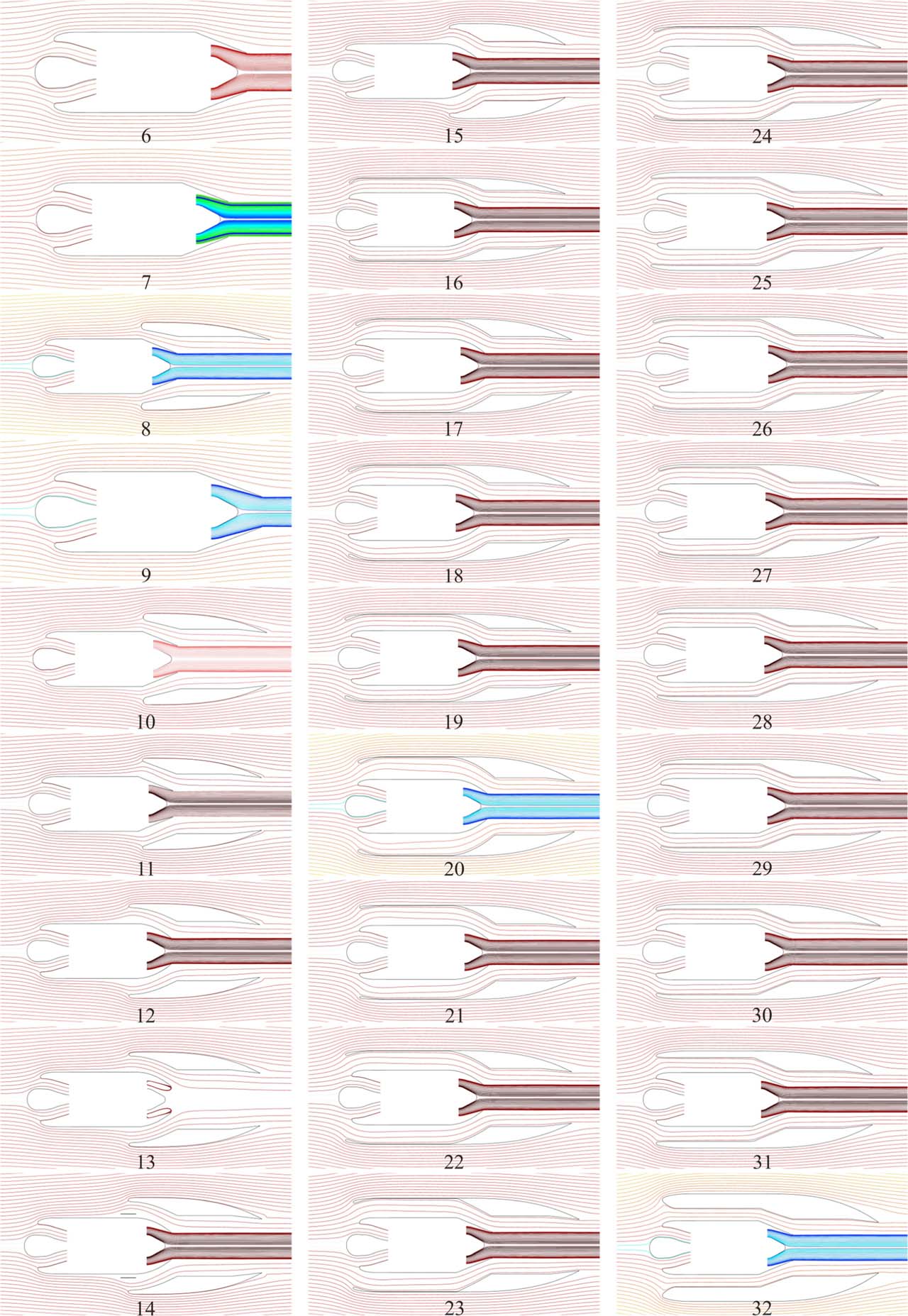
Fig. 14.
Pathline patterns for the configurations considered (α* = 5).
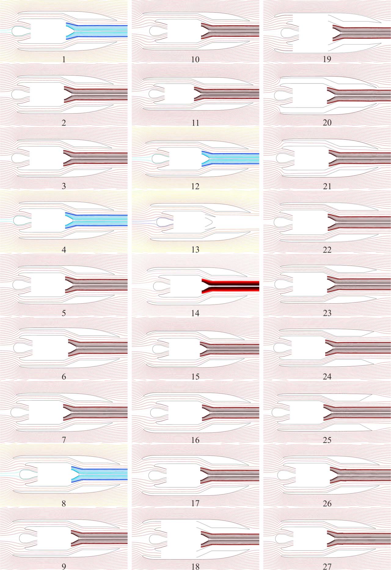
Fig. 15.
Pathline patterns for the configurations considered (α* = 4).
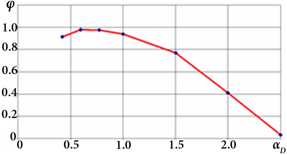
Fig. 16.
Thrust augmentation ratio (φ) vs. the ratio of the common exhaust unit exit area to the mixing chamber area (αD) (configurations 20, 21, 2, 22, 23, 24, 25) (α* = 4).
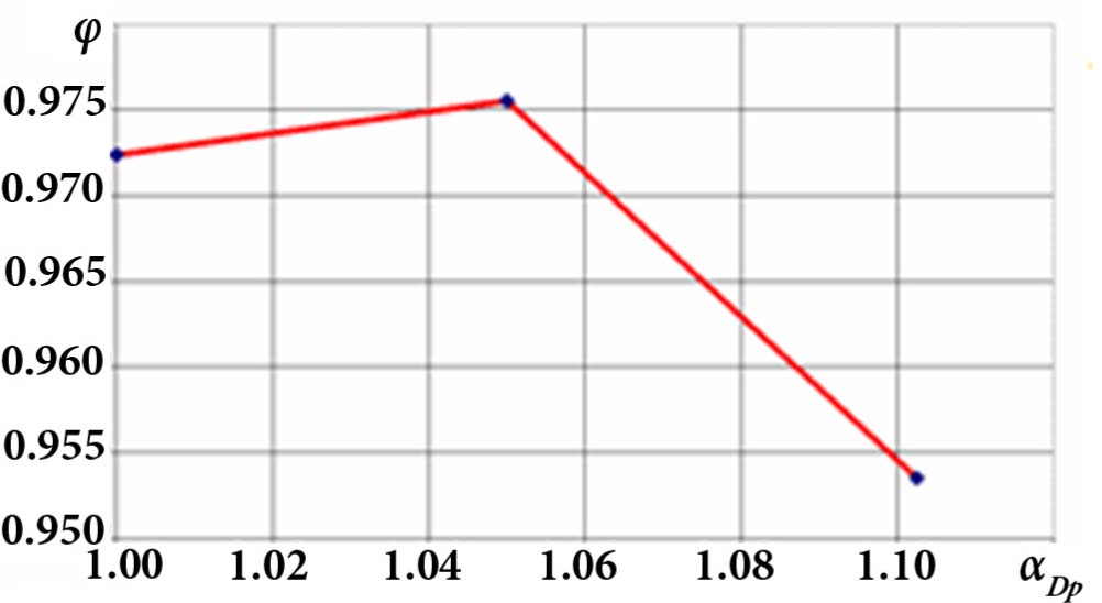
Fig. 17.
Thrust augmentation ratio (φ) vs. the ratio of the primary convergent-divergent nozzle exit area to its throat area (αDp) (configurations 2, 27, 26) (α* = 4).
7.3. Estimation of the influence of the primary nozzle pressure ratio πN
According to Alperin’s 1D theory [23, 24], the influence of the primary nozzle pressure ratio πN on the thrust augmentation ratio (for the first, or subsonic, solution) within the Mach number range [0.4...1.4] is practically negligible and does not allow any considerable thrust increase to be obtained. In order to check this statement, computations were performed in ANSYS Fluent 2024R1 for the modified configurations 28 and 29 (based on configuration 2 for α* = 4) and for the corresponding configurations without an ejector, 28w and 29w.
For configurations 28 and 28w it was assumed that πN = 3 and R1p = 29.28 mm; for configurations 29 and 29w, πN = 5 and R1p = 22.68 mm.
The mesh parameters corresponded to mesh 3 (10 × 0.20 mm).
The boundary conditions were set as described in Section 5.3, except for the following, which were set for InletPrimary (type = pressure-inlet) in the Momentum tab of the Pressure Inlet dialog window:
Gauge Total Pressure (pascal) = 3*pa (for configurations 28 and 28w);
Gauge Total Pressure (pascal) = 5*pa (for configurations 29 and 29w),
These computations yielded the fields shown in Fig. 18, together with the nozzle thrust (with and without the ejector) and the thrust augmentation ratio for the two values of the primary nozzle pressure ratio πN (Fig. 19).
Alperin’s statement has thus been confirmed, at least for M∞ = 0.6: variation of πN has practically no influence on the thrust augmentation ratio within the Mach number range [0.4...1.4] for the first solution, in which the speed at the exit cross-section of the mixing chamber is subsonic, and the values of the thrust augmentation ratio themselves are close to unity, so that no increase in engine thrust can be obtained by installing an ejector nozzle.
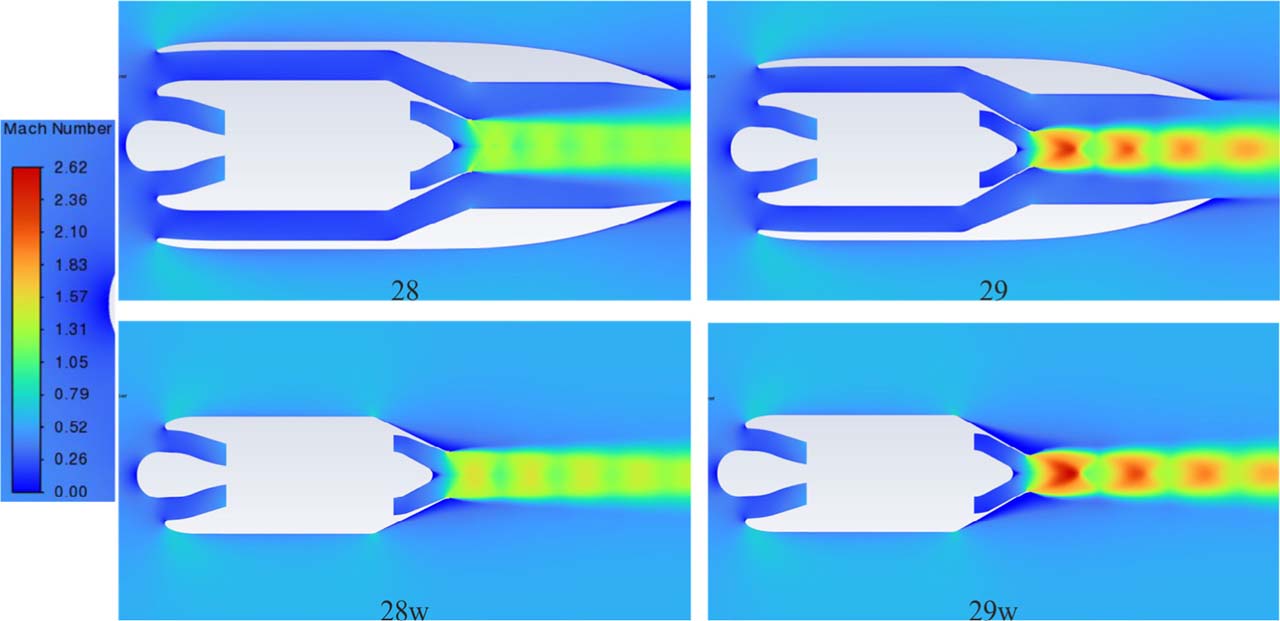
Fig. 18.
Fields of Mach number for configurations 28, 28w, 29 and 29w (α* = 4).
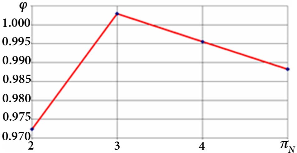
Fig. 19.
Thrust augmentation ratio (φ) vs. primary nozzle pressure ratio πN (the value at the point πN = 4 was interpolated).
8. CONCLUSIONS
In 2D computations of various engine configurations with annular and nose air intakes for the secondary air flow, performed in ANSYS Fluent 2024R1 for ratios of the mixing chamber cross-sectional area to the primary nozzle exit area α* = 4 and 5, it was not possible to reach the design secondary flow rate at the entrance to the mixing chamber required by Alperin’s second solution, because some factor braked the secondary flow in front of the mixing chamber exit. Thrust therefore cannot be increased by applying an ejector nozzle.
Even when the secondary flow rate in front of the ejector nozzle was set explicitly, using Alperin’s 1D theory for the second solution, the flow at the exit of the mixing chamber remained subsonic, which corresponds to the first solution.
By varying the exit area of the convergent exhaust unit located behind the mixing chamber, it was found that the factor braking the secondary flow in front of the exit of the mixing chamber is the contraction of the common exhaust unit. If the exhaust unit is made cylindrical or divergent, high values of the air flow rate and of the Mach number of the secondary flow at the entrance to the mixing chamber are easily obtained. The thrust augmentation ratio then decreases, however, and its maximum value remains below unity, so that the thrust of an engine with an ejector nozzle cannot be increased at the specified Mach number M∞ = 0.6.
It was found that, as the ratio of the exit area of the primary convergent-divergent nozzle to its throat area increases, the thrust augmentation ratio decreases, its maximum value corresponding to a convergent nozzle. The use of a convergent-divergent nozzle for the specified parameters of the primary flow is therefore unjustified.
The 2D computations in ANSYS Fluent 2024R1 confirmed Alperin’s statement, at least for M∞ = 0.6: variation of πN has practically no influence on the thrust augmentation ratio within the Mach number range [0.4...1.4] for the first solution, in which the speed at the exit cross-section of the mixing chamber is subsonic, and the values of the thrust augmentation ratio themselves are close to unity, so that no increase in engine thrust can be obtained by installing an ejector nozzle.
The absence of effective mixing is an additional factor preventing a thrust increase from being obtained.
Abbreviations
- CFD
Computational Fluid Dynamics
- GCI
Grid Convergence Index
- UAV
Unmanned Aerial Vehicles
- AR
Asymptotic range
- Cp
coefficient of heat conductivity
- CR
Convergence ratio
- Δ
Difference between parameters
- e
Relative error
- fex
Richardson extrapolated value
- h
Representative cell size
- hreq
Optimal cell size
- L
Total length of engine
- M∞
flight Mach number
- P
Parameter
- p
Apparent order of approximation
- R
Middle radius of engine
- r
Grid refinement factor
- s
Sign
- α*
Ratio of mixing chamber area to the primary nozzle exit area
- αD
Ratio of exit area of the common exhaust unit to mixing chamber cross-section area
- αDp
Ratio of exit area of the primary nozzle to its throat area
- πN
primary nozzle pressure ratio
- φ
Ratio of ejector nozzle thrust to thrust of isolated primary nozzle at the same mode