
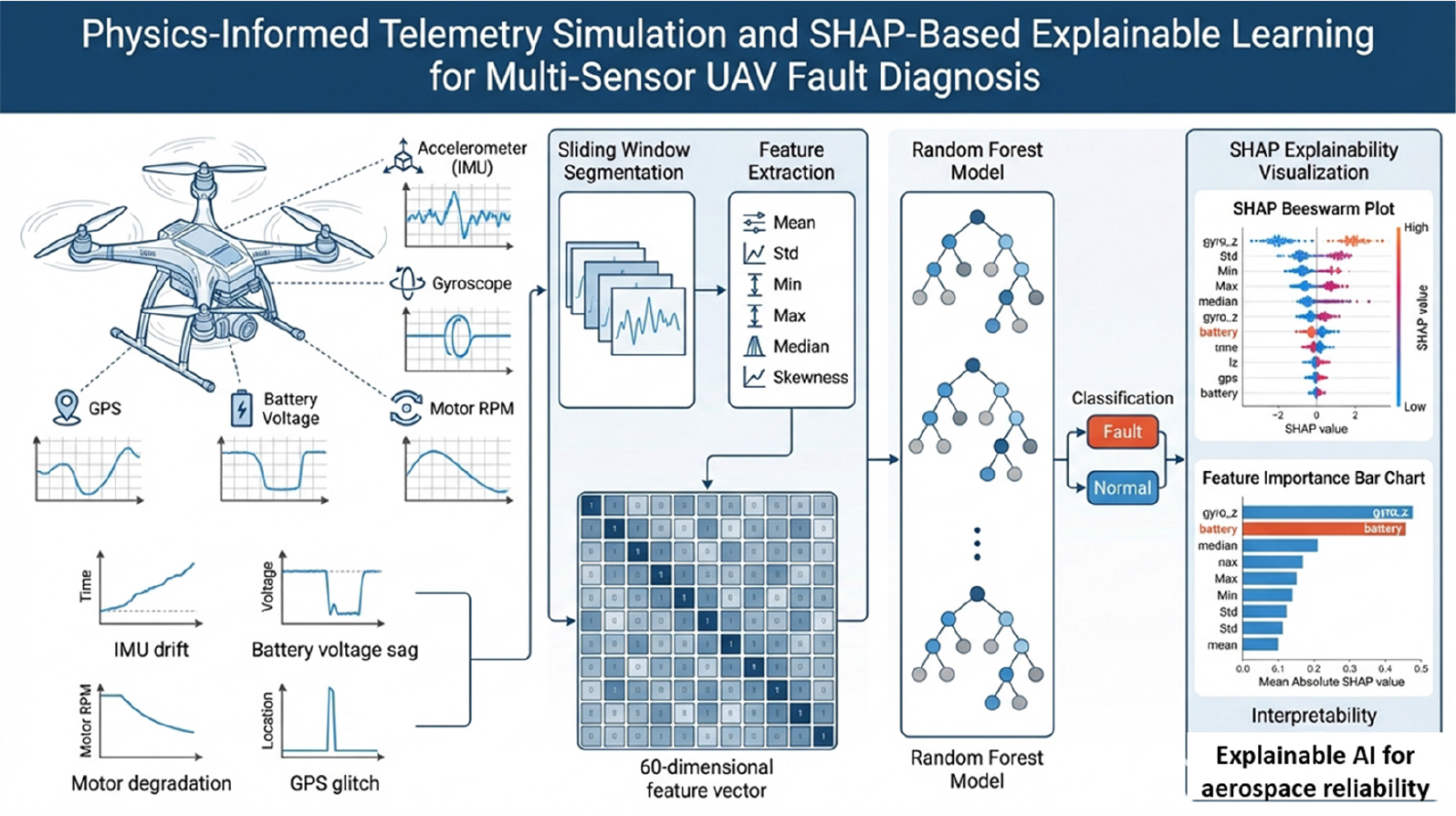
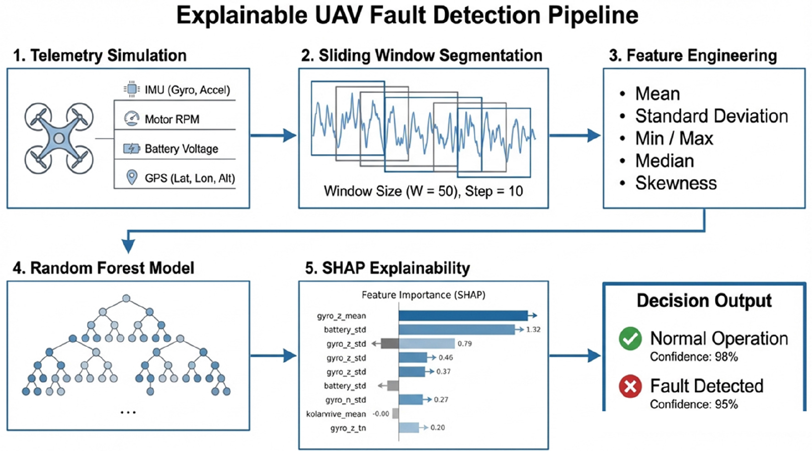
Fig. 1.
Full pipeline diagram illustrating the data flow from simulated UAV telemetry to windowing, feature engineering, machine-learning-based fault detection, and SHAP explainability.
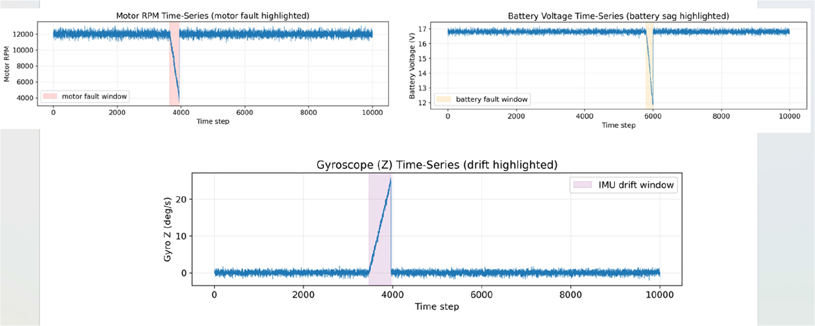
Fig. 2.
Representative examples of simulated UAV telemetry under nominal and faulty operating conditions. (a) Motor RPM time-series exhibiting stable rotational speed during healthy operation followed by a gradual, fault-induced degradation characteristic of propulsion-system weakening. (b) Battery voltage profile showing a distinct sag region, where a controlled drop in cell voltage emulates accelerated discharge or power-system instability, (c) Gyro-z angular rate signal illustrating progressive IMU drift, with a monotonic bias accumulation that reflects thermomechanical sensor degradation.

Fig. 3.
Window-level fault annotation timeline illustrating the segmentation of the multivariate telemetry stream into overlapping analysis windows. Each window is categorized as normal (green) or faulty (red) based on the presence of any injected anomaly within its temporal span. This visualization highlights the distribution and duration of simulated fault events and demonstrates how the windowing strategy preserves both short-term disturbances and gradually evolving subsystem degradations.
Table 1.
Extracted statistical features generated for each of the ten sensor channels (60 features in total).
| Sensor Channel | Extracted Features (6 per channel) |
|---|---|
| accel_x | accel_x _mean, accel_x_std, accel_x_min, accel_x_max, accel_x_median, accel_x_skew |
| accel_y | accel_y _mean, accel_y_std, accel_y_min, accel_y_max, accel_y_median, accel_y_skew |
| accel_z | accel_z_mean, accel_z_std, accel_z_min, accel_z_max, accel_z_median, accel_z_skew |
| gyro_x | gyro_x_mean, gyro_x_std, gyro_x_min, gyro_x_max, gyro_x_median, gyro_x_skew |
| gyro_y | gyro_y_mean, gyro _y_std, gyro _y_min, gyro_y_max, gyro _y _median, gyro_y_skew |
| gyro_z | gyro_z_mean, gyro_z_std, gyro_z_min, gyro_z_max, gyro_z_median, gyro_z_skew |
| motor_rpm | motor_rpm_mean, motor_rpm _std, motor_rpm _min, motor_rpm_max, motor_rpm_median, motor_rpm_skew |
| battery | battery _mean, battery_std, battery_min, battery_max, battery_median, battery_skew |
| gps_lat | gps_lat_mean, gps_lat_std, gps_lat_min, gps_lat_max, gps_lat_median, gps_lat_skew |
| gps_lon | gps_lon_mean, gps_lon_std, gps_lon_min, gps_lon_max, gps_lon_median, gps_lon_skew |
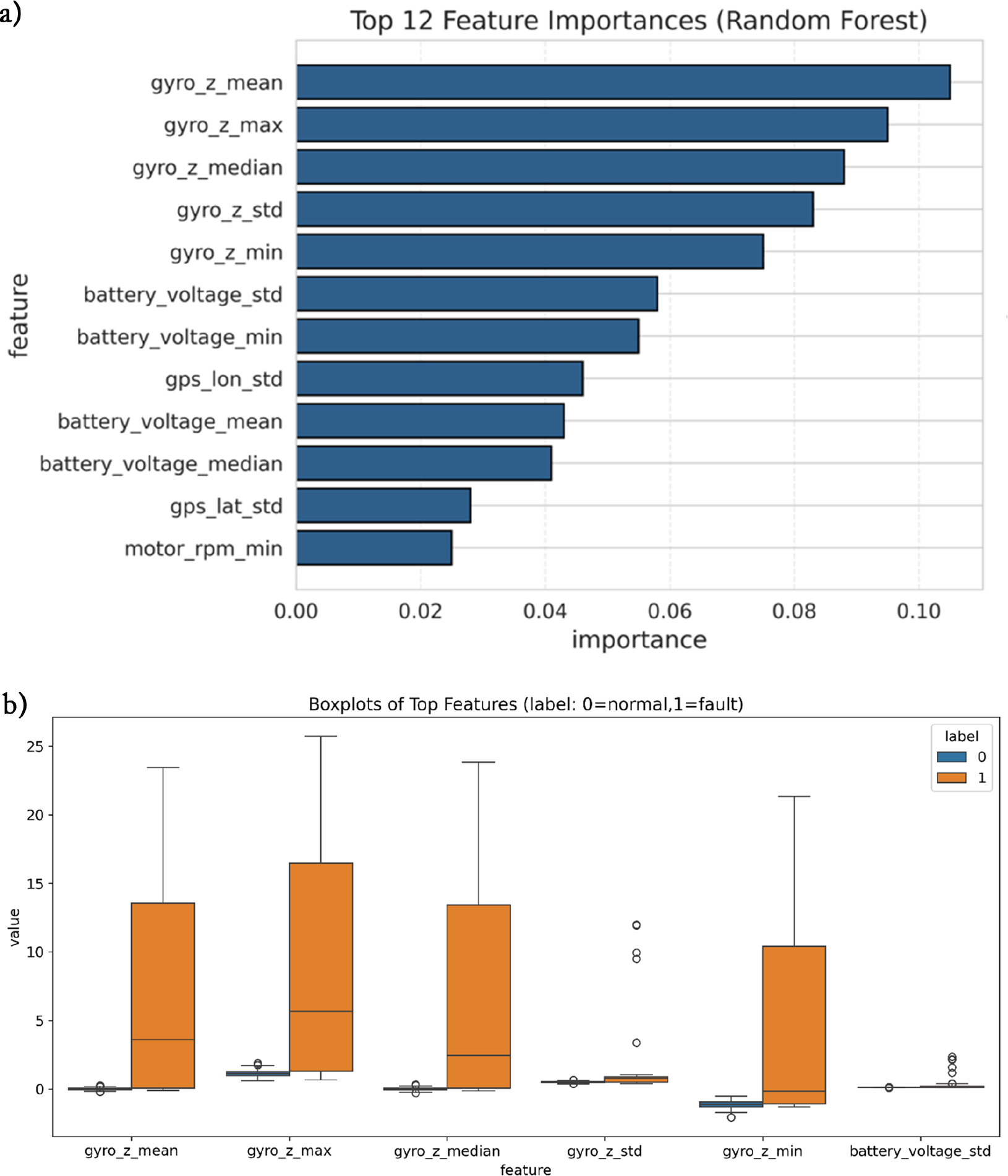
Fig. 4.
Feature-level characterization of the most discriminative signals for UAV fault classification. (a) Ranked feature importance scores computed using the Random Forest model, highlighting the dominant influence of gyro_z-related statistics (mean, max, median, and standard deviation) and battery-voltage variability, which collectively encode the strongest signatures of IMU drift and power-system instability. (b) Boxplot distributions of the top contributing features for normal (label 0) and faulty (label 1) windows. Fault conditions exhibit pronounced shifts in central tendency and dispersion, particularly in gyro_z_mean, gyro_z_max, and battery_std, demonstrating clear statistical separability between healthy and anomalous operating states.
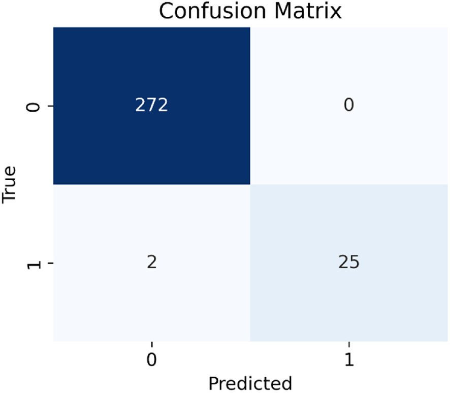
Fig. 5.
Confusion matrix illustrating the classification performance of the Random Forest model on the test dataset. The results indicate strong discrimination between nominal and faulty telemetry windows, with a high proportion of true negatives and true positives and limited misclassification. These findings support the effectiveness of the engineered statistical feature representation and ensemble-based classification strategy for detecting diverse UAV subsystem anomalies under the defined simulation conditions.
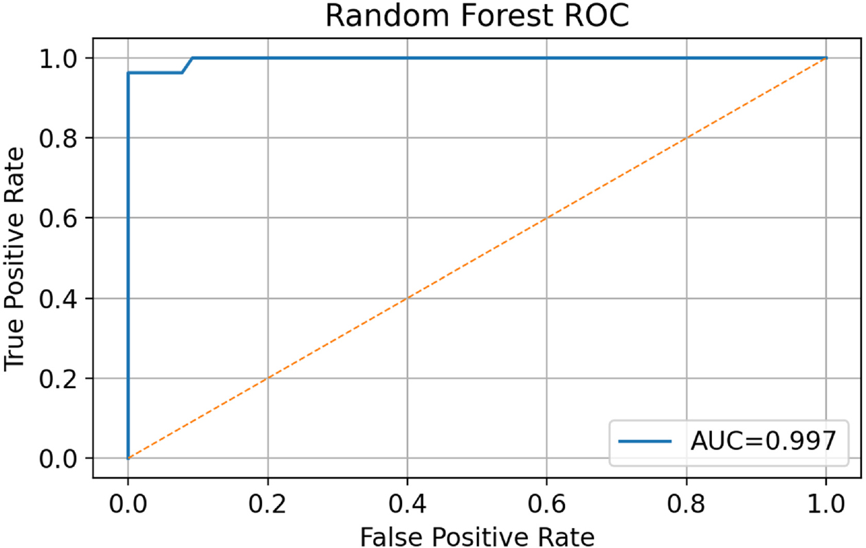
Fig. 6.
Receiver Operating Characteristic (ROC) curve for the Random Forest classifier, illustrating its strong discriminative capability across varying decision thresholds. The model achieves an Area Under the Curve (AUC) of 0.997, indicating near-perfect separability between normal and faulty telemetry windows and confirming the effectiveness of the engineered feature set and ensemble-learning architecture.
Table 2.
Classification report summarizing precision, recall, and F1-score for normal and faulty windows.
| Class | Precision | Recall | F1-Score | Support |
|---|---|---|---|---|
| Normal (0) | 0.99 | 1.00 | 1.00 | 272 |
| Fault (1) | 1.00 | 0.93 | 0.96 | 27 |
| Overall Accuracy | – | – | 0.9933 | 299 |
| Macro Avg | 1.00 | 0.96 | 0.98 | 299 |
| Weighted Avg | 0.99 | 0.99 | 0.99 | 299 |
Table 3.
Performance comparison of different models trained on the same dataset.
| Model | Accuracy (%) | Precision | Recall | F1-Score | Notes |
|---|---|---|---|---|---|
| Logistic Regression | 95.21 | 0.94 | 0.88 | 0.91 | Linear model; struggles with nonlinear drift signatures |
| SVM (RBF) | 97.11 | 0.96 | 0.91 | 0.93 | Strong nonlinear learner; sensitive to feature scaling |
| kNN (k=5) | 94.00 | 0.92 | 0.85 | 0.88 | Local decisions unstable under noisy windows |
| Gradient Boosting | 98.42 | 0.97 | 0.92 | 0.94 | Good performance; higher training cost |
| XGBoost | 98.89 | 0.98 | 0.92 | 0.95 | Excellent for tabular data; slightly higher complexity |
| Random Forest (Proposed) | 99.33 | 1.00 | 0.93 | 0.96 | Best balance of accuracy, robustness, interpretability |
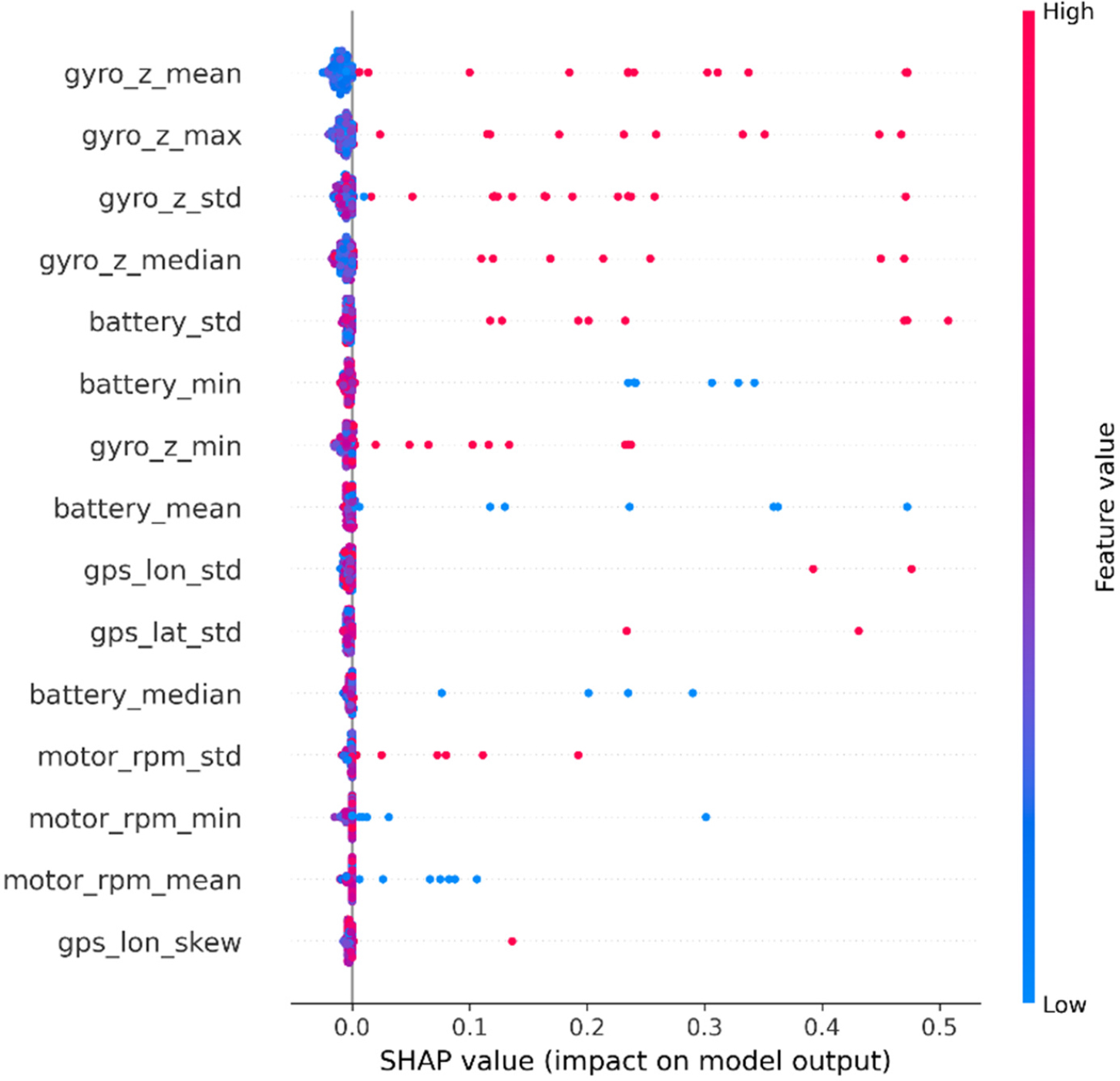
Fig. 7.
SHAP summary (beeswarm) plot illustrating the global contribution of each engineered feature to the Random Forest classifier’s decisions. Features related to gyro_z exhibit the highest Shapley magnitudes, confirming their dominant role in capturing IMU drift, while battery-voltage descriptors and GPS-variability metrics provide additional discriminative information for identifying sag events and positional anomalies. The colour gradient reflects the relative feature values within each window, enabling direct interpretation of how specific sensor behaviours influence fault likelihood.
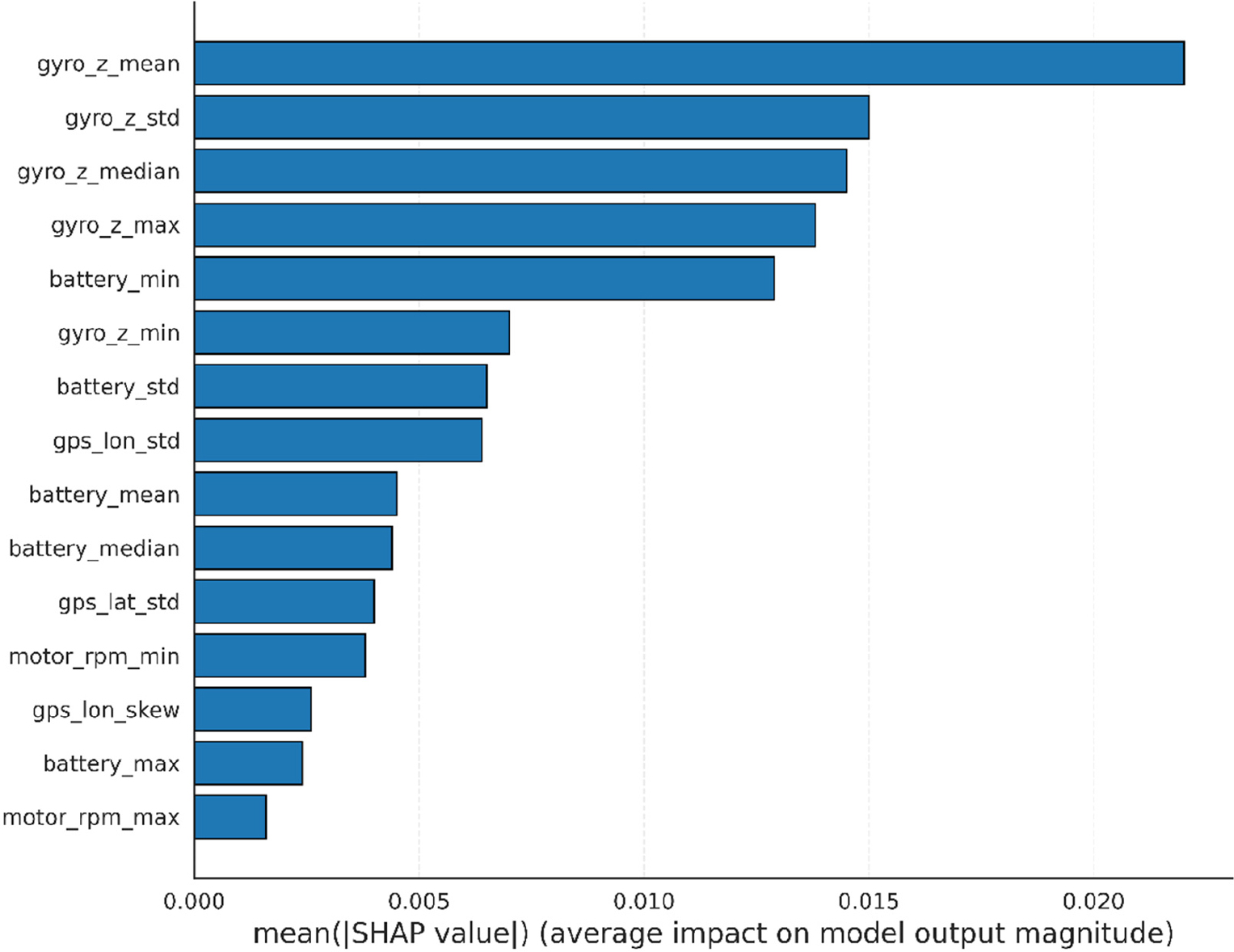
Fig. 8.
SHAP global feature-importance ranking computed from the mean absolute Shapley values across all test samples. Features associated with gyro_z exhibit the highest contributions, highlighting their dominant role in detecting IMU drift, while battery-voltage statistics and GPS-variability descriptors provide secondary yet meaningful influence on the classifier’s decisions. The ranking confirms that the model’s fault predictions are driven by physically interpretable sensor behaviours rather than noise or spurious correlations.
Table 4.
Representative comparison with existing UAV fault-detection approaches.
| Study / Approach | Dataset Type | Model Type | Explainability | Reported Accuracy |
|---|---|---|---|---|
| Threshold-based methods [1–5] | Real flight data | Rule-based | None | 70–85% |
| SVM-based detection [14,16] | Laboratory IMU datasets | SVM | None | 85–92% |
| Deep CNN (single-sensor) [18] | Vibration data | CNN | Limited | 92–96% |
| LSTM-based anomaly detection [19–21] | Time-series telemetry | LSTM | None | 95–98% |
| Proposed framework (RF + SHAP) | Simulated multimodal telemetry | Random Forest | SHAP-based | 99.3% |
| Symbol | Description |
|---|---|
| N | Total number of telemetry samples |
| W | Sliding window length |
| s | Sliding window step size |
| X | Window-level feature matrix |
| y | Binary window-level labels (fault / normal) |
| F | Number of features extracted per window |
| T | Number of trees in the Random Forest |
| Predicted class labels | |
| p | Predicted fault probability |
| SHAP (·) | SHAP value computation operator |
| M | Number of training samples |
| S | Number of test samples |