
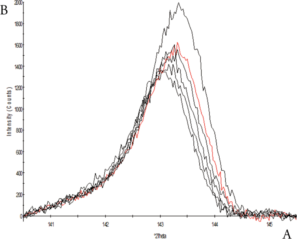
Figure 1.
Profiles of diffraction lines obtained at different angles of incidence ψ of the beam of X-ray waves: (A) horizontal axis – angle 2Θ; and (b) vertical axis – intensity of X-ray diffraction.
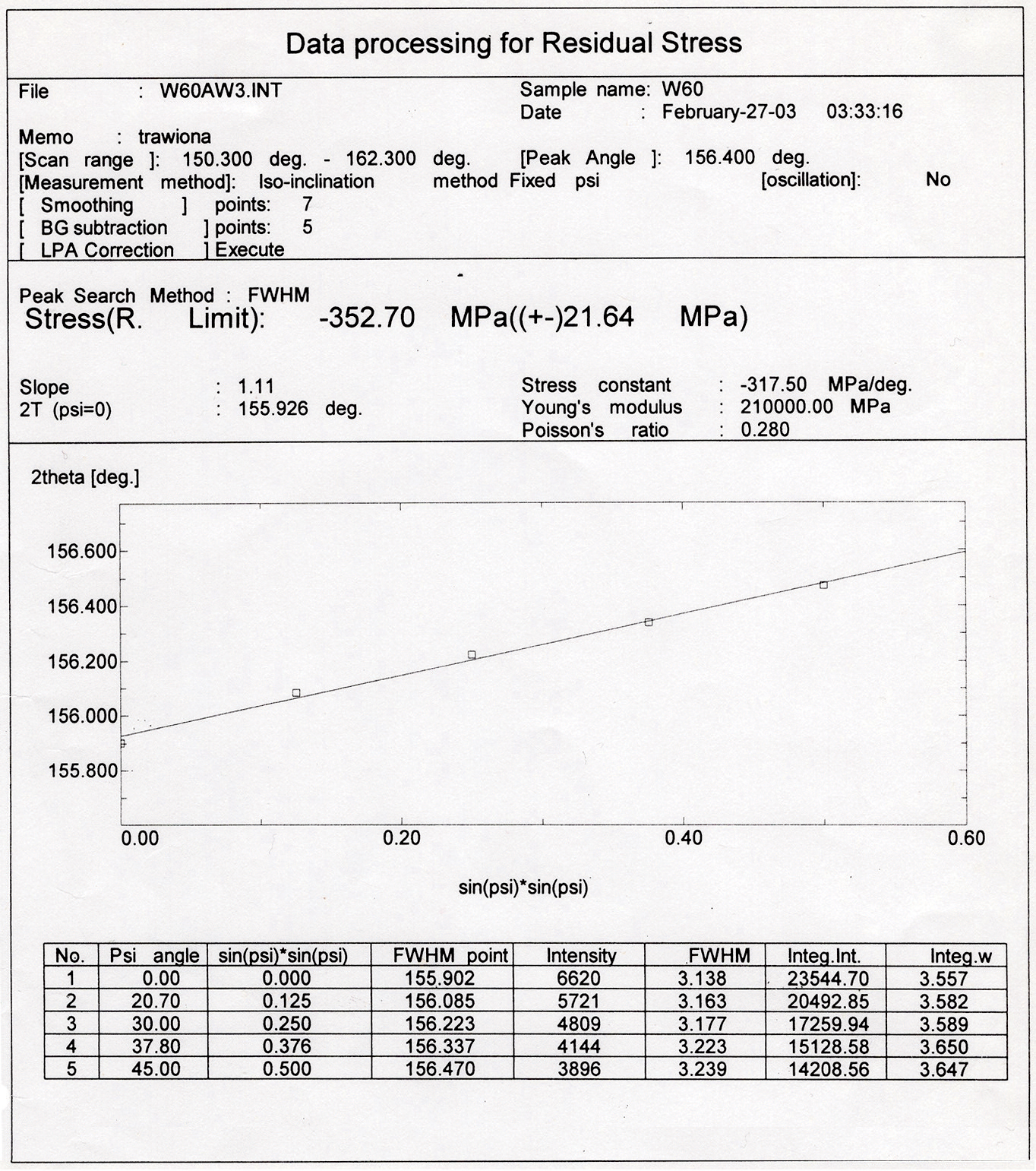
Figure 2.
Report on the measurement of residual stresses using the X-ray method, using the PSWF-3M device from the Rigaku Company: Young’s modulus E = 210,000.0 MPa and Poisson’s ratio ν = 0.280.

Figure 3.
PEEN-IMP device for pneumatic peening (patent PL204718).
Table 1.
Measurements of stresses σ MPa as a function of distance d mm from the surface.
| LP | Distance from the surface d mm | Hardness HRC | Steel shot N 1,2,3,4 | Stresses σ MPa |
|---|---|---|---|---|
| 1 | 0.000 | 35 | 1 | −506.37 |
| 2 | 0.079 | 35 | 1 | −465.59 |
| 3 | 0.127 | 35 | 1 | −390.06 |
| 4 | 0.194 | 35 | 1 | −397.08 |
| 5 | 0.241 | 35 | 1 | −244.17 |
| 6 | 0.299 | 35 | 1 | −209.32 |
| 7 | 0.399 | 35 | 1 | −232.61 |
| 8 | 0.456 | 35 | 1 | −172.24 |
| … | ||||
| 25 | 0.000 | 30 | 2 | −448.40 |
| 26 | 0.046 | 30 | 2 | −540.25 |
| 27 | 0.106 | 30 | 2 | −571.50 |
| 28 | 0.150 | 30 | 2 | −547.69 |
| 29 | 0.210 | 30 | 2 | −527.38 |
| 30 | 0.258 | 30 | 2 | −514.13 |
| 31 | 0.315 | 30 | 2 | −427.26 |
| 32 | 0.340 | 30 | 2 | −354.94 |
| 33 | 0.396 | 30 | 2 | −305.50 |
| … | ||||
| 70 | 0.000 | 45 | 3 | −682.34 |
| 71 | 0.051 | 45 | 3 | −602.13 |
| 72 | 0.111 | 45 | 3 | −615.84 |
| 73 | 0.191 | 45 | 3 | −552.10 |
| 74 | 0.206 | 45 | 3 | −395.75 |
| 75 | 0.227 | 45 | 3 | −259.79 |
| 76 | 0.340 | 45 | 3 | −249.39 |
| 77 | 0.393 | 45 | 3 | −293.09 |
| 78 | 0.419 | 45 | 3 | −195.22 |
| … | ||||
| 120 | 0.000 | 50 | 4 | −643.16 |
| 121 | 0.116 | 50 | 4 | −737.91 |
| 122 | 0.166 | 50 | 4 | −745.57 |
| 123 | 0.220 | 50 | 4 | −509.45 |
| 124 | 0.284 | 50 | 4 | −394.01 |
| 125 | 0.347 | 50 | 4 | −432.17 |
| 126 | 0.401 | 50 | 4 | −321.01 |
| 127 | 0.462 | 50 | 4 | −254.92 |
| 128 | 0.565 | 50 | 4 | −261.30 |
Table 2.
Coefficients of the regression function calculated by the program for the results of measurements.
| Variable number | Regression coefficient | Std. Error of reg. coeff. | Computed T-value | |
|---|---|---|---|---|
| (c1) | 1 | −0.845537E+02 | 303.47275 | −0.279 |
| (c7) | 7 | −0.865059E+01 | 1.82461 | −4.741 |
| (c6) | 6 | 0.259431E+02 | 52.86755 | 0.491 |
| (c2) | 2 | −0.109254E+03 | 26.07856 | −4.189 |
| (c10) | 10 | 0.798438E+02 | 14.47331 | 5.517 |
| (c9) | 9 | 0.160997E+01 | 0.35632 | 4.518 |
| (c3) | 3 | −0.114981E+03 | 60.96822 | −1.886 |
| (c5) | 5 | 0.138582e+02 | 7.15698 | 1.936 |
| (c8) | 8 | 0.493962E+03 | 288.88644 | 1.710 |
| (c0) | 0.168799E+04 |
Table 3.
Statistical evaluation of the obtained regression function using the statistical parameters R2 (the square of the multiple correlation coefficient) and F (Snedecor’s test).
| STEP 9 |
| VARIABLE ENTERED..... 8 |
| (FORCED VARIABLE) |
| SUM OF SQUARES REDUCED IN THIS STEP.... 18743.844 |
| PROPORTION REDUCED IN THIS STEP........ 0.006 |
| CUMULATIVE SUM OF SQUARES REDUCED...... 2162765.250 |
| CUMULATIVE PROPORTION REDUCED.......... 0.741 OF 2919265.000 |
| FOR 9 VARIABLES ENTERED |
| MULTIPLE CORRELATION COEFFICIENT... 0.861 |
| (ADJUSTED FOR D.F.)........... 0.851 |
| SQUARE MULTIPLE CORRELATION COEFFICIENT ⊠ 0.741 |
| F-VALUE FOR ANALYSIS OF VARIANCE... 37.483 |
| STANDARD ERROR OF ESTIMATE......... 80.069 |
| (ADJUSTED FOR D.F.)........... 82.716 |
Table 4.
Values of residual stresses σ as a function of changing the X1 depth extending into the surface layer calculated by the FUNVAL3.EXE program.
| Type of function - NATURAL -N- | ||
| Values of Bi coefficients in the calculated function | ||
| B0= 0.1688E+04, B1= −0.8455E+02, B2= −0.1093E+03, | ||
| B3= −0.1150E+03 | ||
| B12= 0.1386E+02, B13= 0.2594E+02, B23= −0.8651E+01, | ||
| B11= 0.4940E+03, B22= 0.1610E+01, B33= 0.7984E+02 | ||
| NUMBER OF POINTS N = 8 | ||
| Values of X1, X2, X3 variables at set points | ||
| X1 | X2 | X3 |
| 0.000 | 35.0000 | 1.0000 |
| 0.1000 | 35.0000 | 1.0000 |
| 0.2000 | 35.0000 | 1.0000 |
| 0.3000 | 35.0000 | 1.0000 |
| 0.4000 | 35.0000 | 1.0000 |
| 0.5000 | 35.0000 | 1.0000 |
| 0.6000 | 35.0000 | 1.0000 |
| 0.7000 | 35.0000 | 1.0000 |
| 0.8000 | 35.0000 | 1.0000 |
| Xi depth and Yi function values at set points | ||
| No. | Xi | Yi |
| 1 | 0.000 | −501.1677 |
| 2 | 0.1000 | −454.0123 |
| 3 | 0.2000 | −396.5508 |
| 4 | 0.3000 | −329.2101 |
| 5 | 0.4000 | −251.9901 |
| 6 | 0.5000 | −164.8909 |
| 7 | 0.6000 | −67.9124 |
| 8 | 0.7000 | 38.9453 |
| 9 | 0.8000 | 155.6822 |
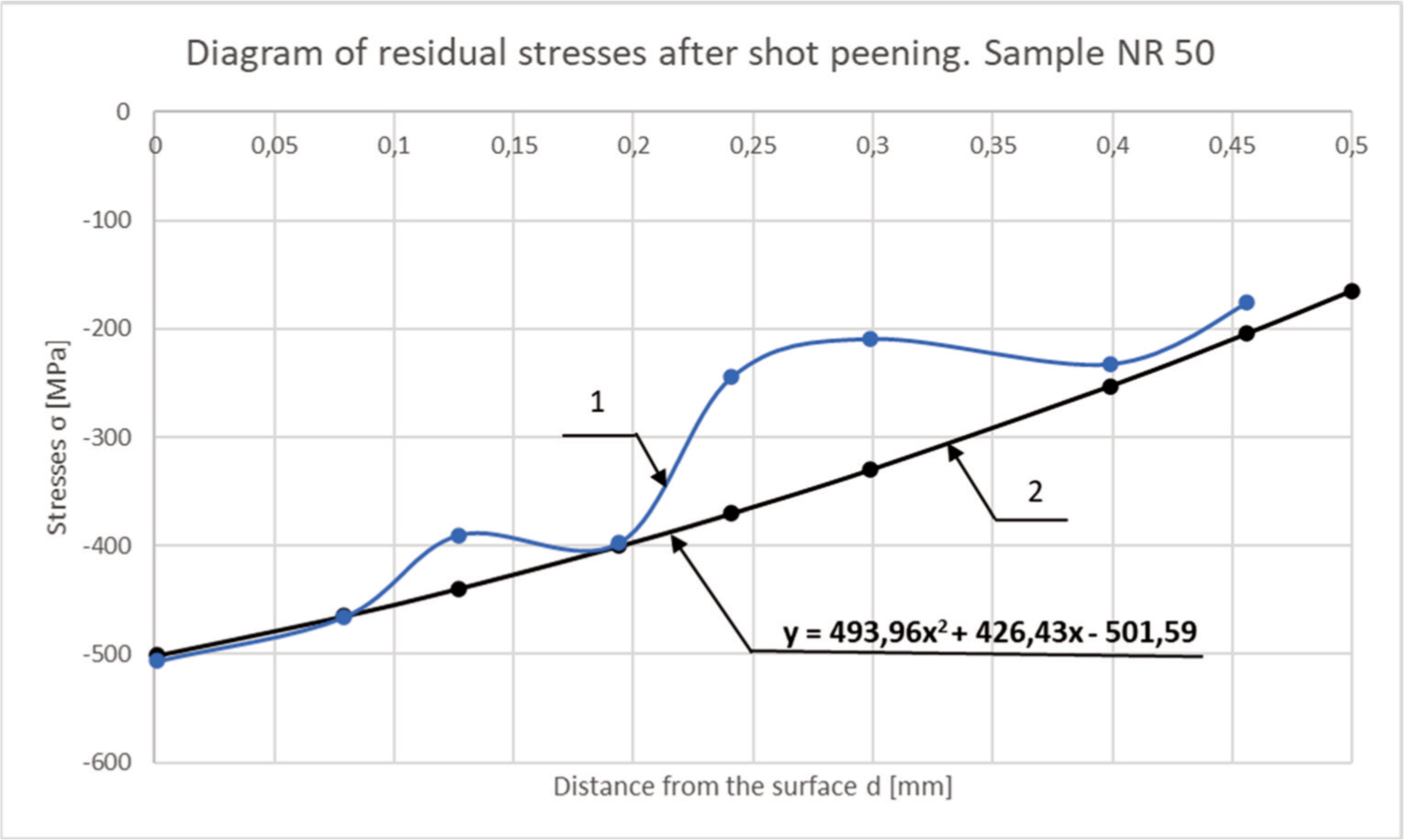
Figure 4:
Graph of residual stress distribution in the sample after shot peening:
sample NR50 (HRC, 35 MPa), shot N = 1,
curve 1 – measured distribution of residual stresses, to a depth of 0.5 mm,
curve 2 – distribution of residual stresses created by REGSTEP.EXE, represented by the equation: y = 493,96x2 + 426,43x_501,59.