Calibration of the dynamic replacement column forming model with the softening of the soil and columns stiffness increase

1. Introduction

Dynamic replacement is one of the methods of ground improvement within geotechnical engineering [1]. It consists in forming aggregate columns in soft soil because of several drops of pounder (usually over 10 tons) from a height of up to 25 m. The columns obtained in this way are characterized by lengths of up to 5 m and diameters depending on the diameters of the pounders (D _p) used – approximately 1.5–2D _p [2]. During the formation of columns, the operator does not have direct control over their length and diameters, although skilful handling of the discharge height and the size of the crater backfill can affect the obtained column geometry [3]. Bad operations can lead to the formation of the so-called floating columns [4] or almost complete soil replacement [5]. Therefore, an important role is played by trial fields, where the technology of pounder drops is selected depending on the soil and water conditions. An alternative to this procedure may be numerical analyses, preceded by calibration of the model with the results of laboratory and/or field tests. In numerical modelling of this type of problem, mesh models are used [6–8], a combination of mesh and mesh-free models [9,10] and meshless models [11]. Among the mentioned approaches, the authors of the paper attempted to calibrate the model by assuming a combination of classical finite element method (FEM) and the mesh-free method smoothed-particle hydrodynamics (SPH) using the ANSYS LS-Dyna program [12]. The basis was the results of own laboratory tests [13]. The proposed two-dimensional, axially symmetrical model made it possible to simulate about 60% of the column formation process [12]. During the analysis, it was found that the zone of largest displacements modelled with SPH elements was too narrow and the formed column was smaller than observed in the experiments. While smaller column diameters were the reason for the lack of calculations of the full forming process, the analysis of the sinking of the column base showed that it would be impossible to obtain a column based on load-bearing soil. The aforementioned observations were the basis for modifying the model. First, the diameter of the area modelled with SPH elements has been increased. Second, changes in the substrate occurring during the formation of the column, as well as in the column itself, are taken into account.

The specificity of dynamic replacement causes that during the formation of columns (high-energy drops and large displacements in the ground), changes occur in their ground environment. Their nature depends on the type of subsoil. For non-cohesive soils [14] and high in organic parts (peat) [15], the soil is immediately strengthened by compaction (including the organic backbone in the case of peat). In the case of cohesive soils, the water content of which is higher than optimal, a different effect was initially observed – they are softened. As early as 1972, Luis Menard [16] when filing a patent application for the improvement of cohesive soils using the dynamic consolidation method, it states that an increase in water pressure in the pores causes a decrease in the shear strength of the soil, and only after the dispersion of excess water pressure in the pores does, an increase in the physical and mechanical parameters of the soil occur. The waiting time for the substrate to be strengthened depends on the filtration properties of the soil and can be up to several months. Soils with higher cohesiveness require longer waiting times. Led by Kanty and others [13] and Sękowski and others [17] field studies of the impact of column formation on the soil environment have shown that at a distance of up to 1.5 times the diameter of the column during column hammering, the strength parameters of the observed silty soils decrease up to 50% of the original value, but after 30 days, they are even up to 100% higher than the original values. Softening of the subsoil with similar values is confirmed by the research of Yee and Chua [18], and a similar strengthening after the time of consolidation of the substrate is confirmed by studies in the works [19,20]. On the other hand, loose material poured into the crater is compacted during column formation. The forementioned observations concerning the softening of the column surroundings and the increase in the stiffness of the backfill were included in the modified model.

2. Laboratory tests

Detailed information on the study of the influence of column formation during the dynamic replacement process on the surrounding soil, as well as the obtained results, is presented in the previous studies [12,13]. Only the necessary information useful from the point of view of the article is presented here. The laboratory test stand allowed to form a column in dynamic replacement technology. Research was carried out in a box with dimensions of 1 × 1 × 1 m (Figure 1), in which the walls were made of acrylic glass with a thickness of 20 mm, circumferentially improved and in height with steel sections. A 50 mm thick mineral wool introduced at the walls protected against moisture with a foil and dampened vibrations caused during the formation of the column. The improved layer consisted of soft plastic (I _L = 0.7) clay with silt (siCl) with a thickness of 400 mm, lined with very compacted (I _D = 88%) medium sand (MSa) of the same thickness as silty clay (siCl, Figure 1a).

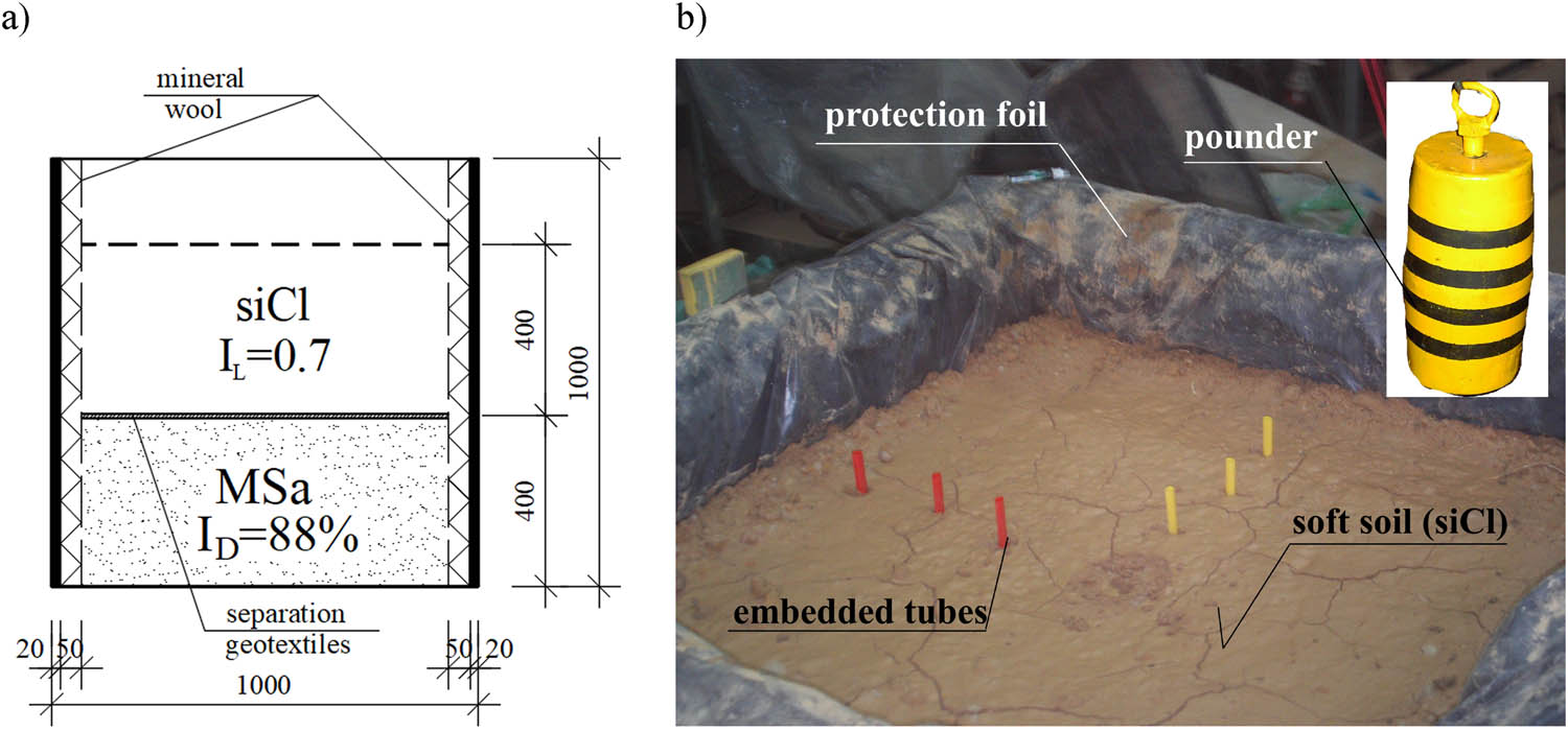
Figure 1

Source: Authors’ contribution.

Columns were formed from basalt aggregate with a fraction of 5–25 mm.

A total of two laboratory tests were carried out, during which the following were performed:

• − measurements of pounder penetrations and masses of aggregate used (test nos. 1 and 2),

• − measurements of horizontal displacements of the ground taking place next to the column (test no. 1),

• − measurements of vertical displacements of the soil (uplift, test no. 1),

• − open-pit mines and column inventory (study nos. 1 and 2).

Additionally, the physical and mechanical parameters of the soil used were determined. They were triaxial compression tests (in unconsolidated and undrained conditions UU) and oedometer tests of soft plastic clay with silt, as well as direct shear box tests of basalt aggregate used for columns and the bottom bearing layer.

In both tests, dynamic replacement columns were formed in the same way, by dropping a barrel-shaped pounder (Figure 1b) with a base diameter of 90 mm, a maximum diameter of 100 mm, a height of 200 mm, and a weight of 10.55 kg, which forced crushed basalt aggregate with a fraction of 5–25 mm into soft plastic clay with silt. The blows were divided into three series. The first one, during which the crater was formed and the first aggregate backfills were applied, consisted of discharges from the height of 0.3, 0.5, 0.7, and 3 × 0.85 m (discharges nos. 1–6). The second (blows nos. 7–32) was the main series, in which the pounder fell from a height of 0.85 m. The last series is to finish off the column head with blows from the height of 0.85, 0.5, 0.3, and 0.15 m. The crater backfills followed discharges no. 3, 4, 5, 6, 33, 34, 35, 36 and after every two blows in the main series. In total, the pounder was dropped 36 times. After individual pounder discharges, the depth of the resulting crater was measured, and the masses and heights of aggregate backfills were recorded.

In total, 22.80 kg of aggregate was used to form the stone column in test no. 1, while in test no. 2, 16.65 kg was used. The columns were 350–390 mm long and had diameters of 150–165 mm (heads) and 220–280 mm (the largest diameter) – Figure 2. Despite repeatable ground conditions and the same pounder discharge heights, the formed columns differ significantly, which is quite characteristic of this method of improvement.

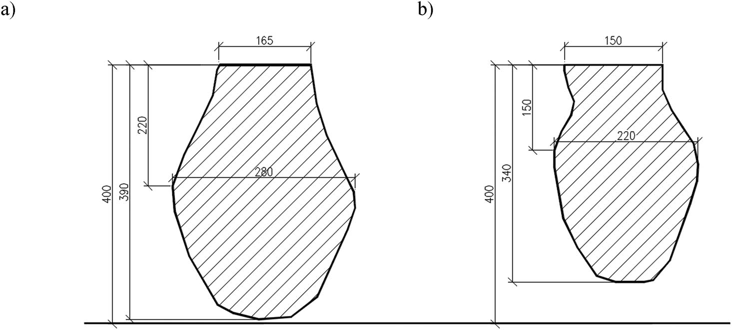
Figure 2

Source: Authors’ contribution.

3. Numerical analysis

3.1. Numerical model

The modified numerical model (Figure 3) was based on the main assumptions of the primary model (FEM + SPH I model) [12]: calculations were carried out in the LS-Dyna program [21], a two-dimensional model (2D) was used in an axially symmetrical state of deformation with a radius (approximately 540 mm) selected so that the horizontal cross-sectional area of the cylindrical cell was equal to the horizontal cross-sectional area of the laboratory box, the whole was modelled by SPH (soft substrate, backfills) and FEM (load-bearing substrate, part of the soft substrate and pounder) – Figure 3a. The volume of stones introduced was identical to that of the original model (FEM + SPH I). The radius of the SPH-modelled zone (R _SPH) has been increased from approximately 220 mm (R _SPH/R _kmax = 1.6, R _kmax – maximum radius of the column – Figure 2) up to approximately 490 mm (R _SPH/R _kmax = 3.5). For computational reasons, it was necessary to leave several FEM elements on the vertical edges of the model. At the junction of the FEM and SPH zones, contact elements (CONSTRAINED_TIE-BREAK) are used [21].

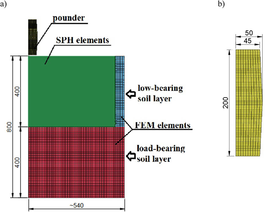
Figure 3

Source: Authors’ contribution.

Standard boundary conditions have been adopted in the form of blocking vertical and horizontal movements on the bottom edge and horizontal movement on the side edges of the model. In addition, due to the damping of vibrations on the walls of the site (use of mineral wool), an edge condition was applied on its numerical side, which did not allow for the reflection of waves reaching it (BOUNDARY_NON_REFLECTING_2D). The thickness of the layers in the model is consistent with that used in laboratory research.

Again, for the modelling of soils, an elastic-perfectly plastic model with the Mohr-Coulomb failure criterion (MAT_173) was used, and its parameters such as the effective angle of internal friction (φ′), effective cohesion (c′), and the shear modulus (G) were determined in laboratory tests and based on the literature (ν). The model assumes undrained conditions, which is characteristic of the issues of very fast loading of cohesive soil [22]. In the first approach (FEM + SPH II model), the attenuation of the substrate was assumed in accordance with the studies of Kanty et al. [13], in which, after making the column, the values of the shear strength in undrained conditions were at the level of 50% of the original value. The calculation assumed a linear reduction of this value during column formation (100% of the soft soil shear strength before the first drop of the pounder and 50% after the last drop, with drops uniformly distributed over time). The authors are aware of the simplification and the qualitative nature of this assumption. In reality, the softening should be simulated, for example, by taking into account the magnitude of plastic strains in the vicinity of the column, after conducting appropriate tests for this purpose (e.g., triaxial compression tests). However, despite the qualitative nature of the assumption, it will be possible to determine whether this approach has an influence on the calculation results.

In the second approach (FEM + SPH III model), both the forementioned softening of the substrate and the increase in the stiffness of the backfill as a function of plastic deformation were assumed. For this purpose, oedometer tests of loose backfill were performed in the range of primary loads of 0–800 kPa, unloading up to approximately 23 kPa and reloading up to 800 kPa and then up to 1200 kPa. Plastic strains were determined based on the unloading curve, for which the elastic and plastic components were identified at individual stress values. The modulus values were determined on the basis of the primary loading curve. The determined plastic deformations for the given load intervals with their corresponding modules, converted to the values of the shear modulus, are shown in Figure 4.

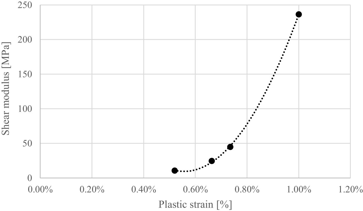
Figure 4

Source: Authors’ contribution.

The pounder (Figure 3b) was modelled using the RIGID model (MAT_20), assuming the parameters of linear elasticity (modulus of elasticity (E) and Poisson’s ratio (ν)) as for steel.

Contact elements (2D_NODE_TO_SOLID) were used between the pounder and the SPH elements, for which the static coefficient of friction (FS) and the dynamic coefficient of friction (FD) were defined with values adopted in this type of issue [23,24].

The values of the parameters of the models used are presented in Table 1.

Table 1

Adopted constitutive models and their parameters.

No.	Element	Constitutive model	Model parameters
1.	Pounder	020-Rigid (model nomenclature in accordance with the ANSYS LS-DYNA conventions)	E = 210 GPa, ν = 0.3, γ = 74 kN/m3
2.	Base layer	173-Mohr-Coulomb	G = 41.7 MPa, φ′ = 33°, c′ = 0 kPa, ν = 0.2, γ = 18 kN/m3
	Medium sand, I D = 88%
3.	Improved layer	173-Mohr-Coulomb	G = 1.39 MPa, Su = 10.2 kPa, ν = 0.31, γ = 18.7 kN/m3
	Silty clay I L = 0.7
4.	DR column aggregates	173-Mohr-Coulomb	G = 6.86 MPa (FEM + SPH II), φ′ = 47°, c′ = 0 kPa, ν = 0.2
			γ = 18 kN/m3
			G = 3.43 – 236 MPa (FEM + SPH III – Figure 4)
5.	Pounder contact elements – SPH elements	N/A	FS = 0.5
			FD = 0.4

Source: Authors’ contribution.

All analyses were performed using the explicit method, i.e., methods based on the explicit scheme are used to integrate the equations of motion, searching for a solution for the next step using the current step, and the state of primary stress was achieved by applying the dynamic relaxation phase.

The calculations were carried out in stages, using the so-called small restart, which allows for the continuity of the model’s calculations. The analysis modelled pounder discharges, its extraction, insertion of the charge, and then its free discharge into the crater, assuming the height of the charge as in laboratory tests. The 36-pounder discharges and 20 portions of aggregates were planned to be divided into 111 stages (36 drops and 36 pounder discharges, 20 backfills and 19 relocations of the aggregate to the drop location above the crater – the first aggregate portion was positioned directly above the crater, while subsequent portions were placed sequentially above it).

The model uses 3060 FEM elements and 44333 SPH elements. The dimensions of the FEM elements were 10 × 10 mm, and the spacing of the SPH elements was 2.5 mm.

3.2. Calculation results and analysis

The modification of the model in the form of increasing the SPH zone allowed for the modelling of the column insertion (FEM + SPH II and III) in its entirety (110 stages). The effect of soil softening modelled during column formation (FEM + SPH II) is visible already at its initial stage (the first four pounder drops) in the form of larger vertical feed drives into the improved substrate (up to 10% – Figure 5, Figure 6a, b), and thus larger pounder’s drives (Figure 6a, b, 7). Initially, the backfill is inserted vertically into the ground (Figure 6a, b) and then the column begins to expand to the sides (from the third backfill, Figures 6c, d, 8a, b). Higher feed drives, reaching up to 20% of the values from the original model in the later stage of formation (Figure 5), result in shifting the maximum diameter of the column to its middle (Figure 6d) and then to the lower part (Figure 8d). In the first model (FEM + SPH I), the maximum diameter of the column occurred in its middle part (Figures 6c, 8c).

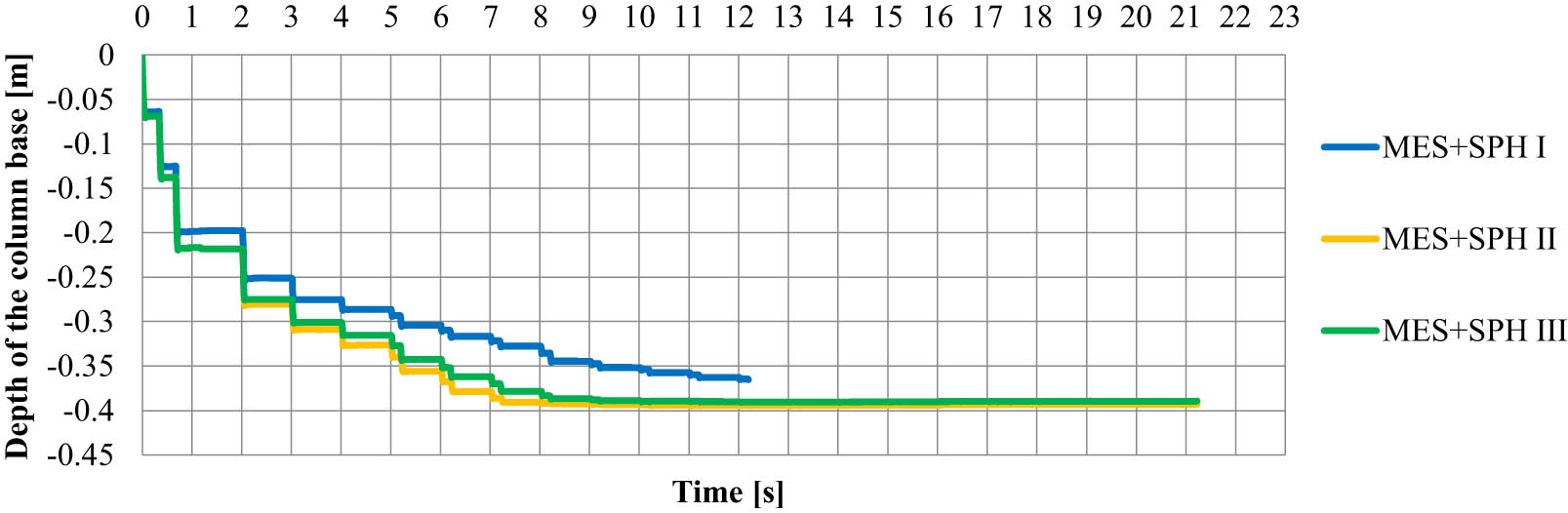
Figure 5

Source: Authors’ contribution.

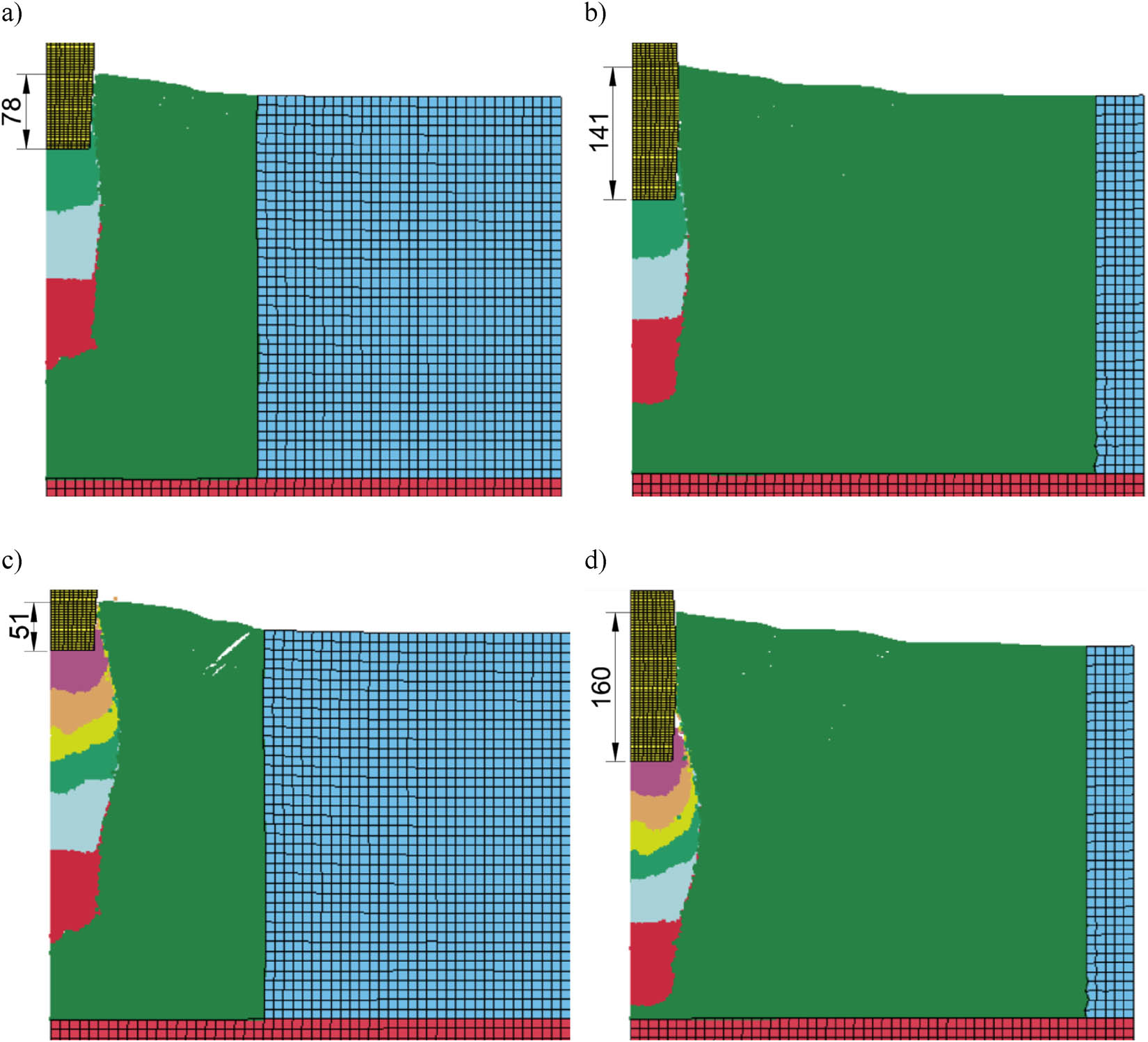
Figure 6

Source: Authors’ contribution.

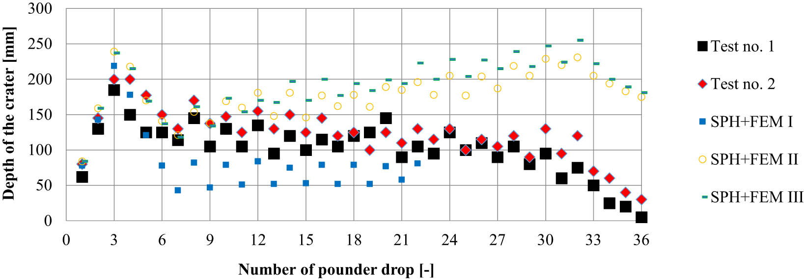
Figure 7

Source: Authors’ contribution.

Due to the instability of the primary model calculation (FEM + SPH I) [12], it is not possible to compare the shape of the columns and the propagation of the compacted aggregate after the 11th backfill (Figure 8c, d).

Modelling the increase in the stiffness of the backfill material (FEM + SPH III) in the initial phase of column formation (until the fourth backfill is driven) has no effect on the feed thrusts into the improved subsoil, and in the subsequent stages, the thrusts obtained in the FEM + SPH III model are up to 5% lower than those observed in the FEM + SPH II model (Figure 5). Greater differences, however, were noticed in the arrangement of the backfills themselves. In the case of the FEM + SPH III model, the backfill is arranged in the shape of semicircles (Figure 9), and in the FEM+SPH II model, with the exception of the first four feeds, the backfill is arranged upward near the column axis (Figure 8b, c, d). This arrangement of the backfills is also observed in the other stages (Figure 10), with the exception of the last three backfills compacted with lower energy (Figure 10c, d).

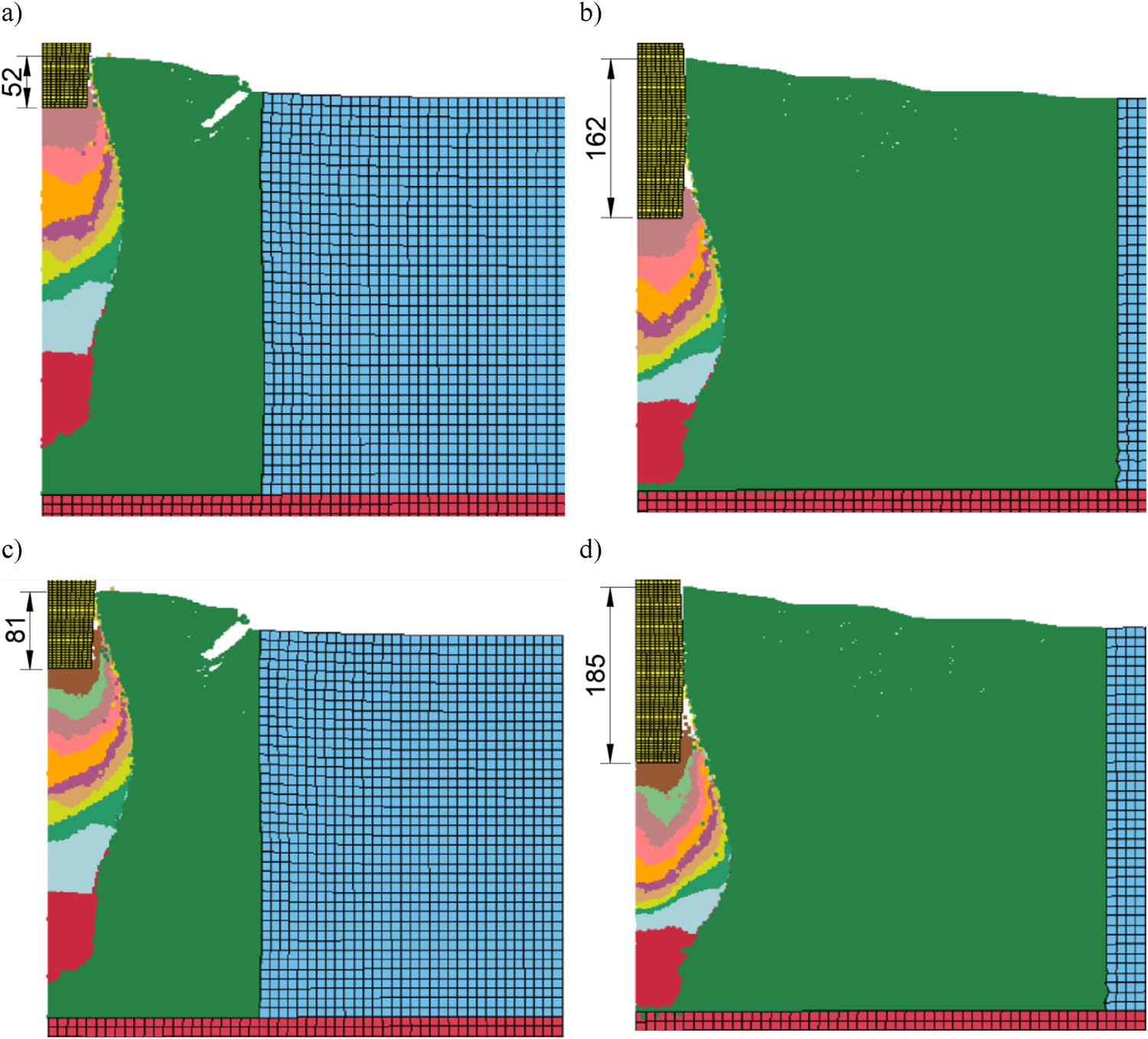
Figure 8

Source: Authors’ contribution.

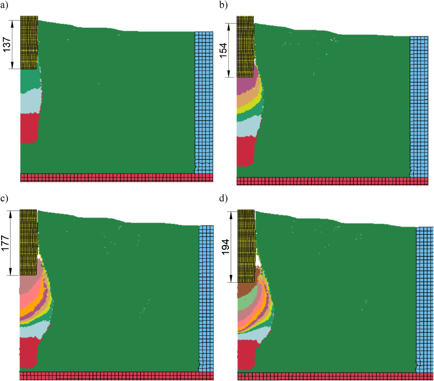
Figure 9

Source: Authors’ contribution.

The numerically obtained columns (FEM + SPH II and III) have practically the same final shapes (Figure 11a). The lower parts of the columns are based on a load-bearing layer (Figure 10c, d) and are similar in shape in their lower parts to column no. 1 from laboratory tests (Figure 11b). The obtained numerical columns have smaller volumes than laboratory columns, which is visible in their upper parts (Figure 11b). The length of the numerical columns was equal to approximately 290 mm (Figure 11a) with the length of the field columns of 340 mm and 390 mm (Figure 2). The reason is that the calculations are identical to the FEM + SPH I. When modifying the FEM + SPH II and III models, it will be necessary to increase the amount of infill to be poured.

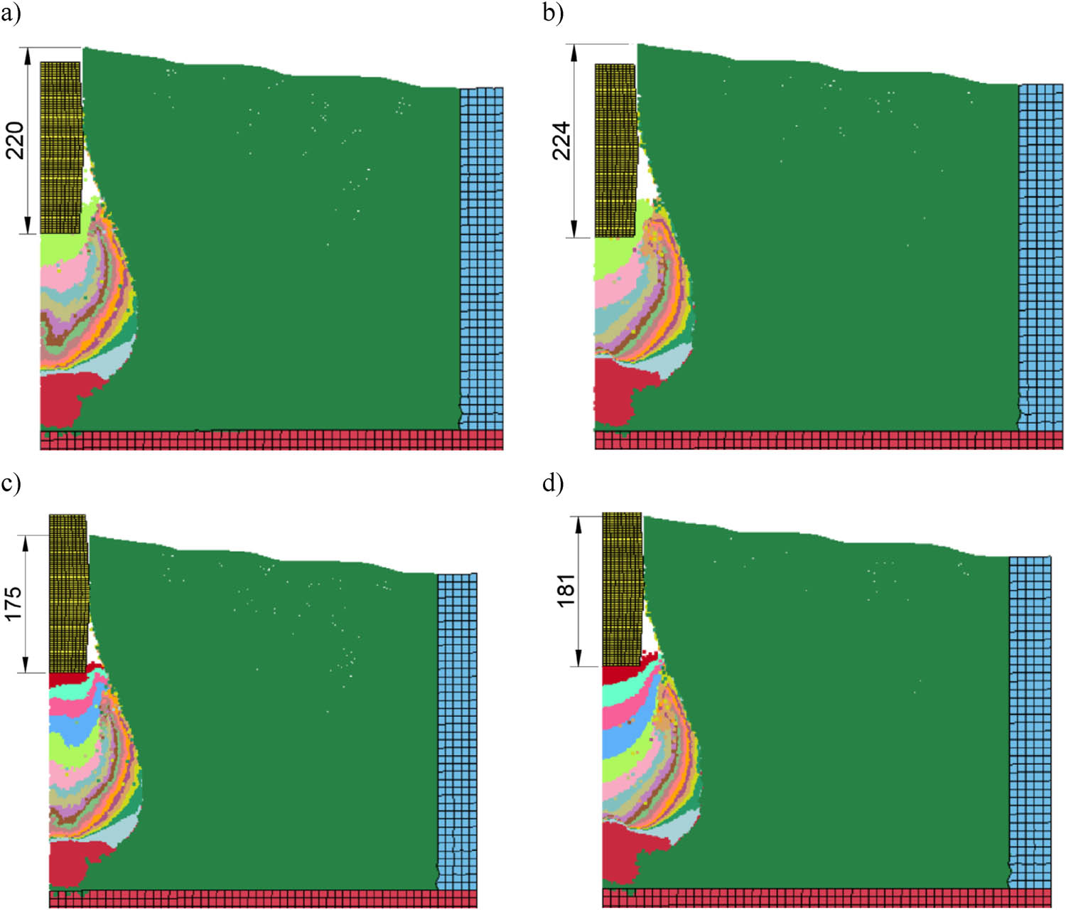
Figure 10

Source: Authors’ contribution.

Figures 12–14 shows a comparison of horizontal displacements of the ground around the column obtained in laboratory tests and numerically at a distance of 150 mm (0.7D _max, D _max – maximum diameter of the column), 200 mm (0.9D _max), and 275 mm (1.25D _max) from the axis of the formed columns. In the case of the immediate vicinity of the column (0.7D _max and 0.9D _max), the obtained maximum horizontal displacements are similar (differences up to 10%, FEM + SPH II and III), but the depth of their occurrence is greater in numerical models (300-320 mm bgl at approx. 250 mm bgl in laboratory tests) – Figures 12–13. At a distance of 275 mm, the horizontal displacements obtained in the FEM+SPH II and III models are more than 100% greater than those observed in laboratory tests. The displacements obtained in the FEM+SPH I model are presented only for information, they are the result of modelling only about 60% of the column forming process.

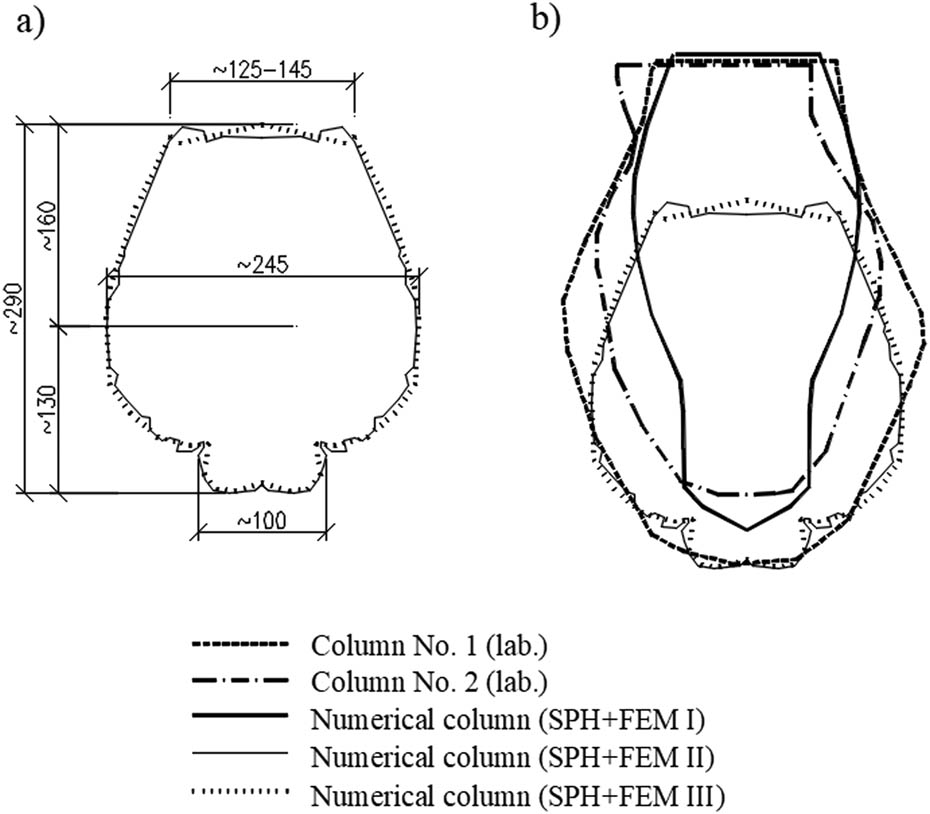
Figure 11

Source: Authors’ contribution.

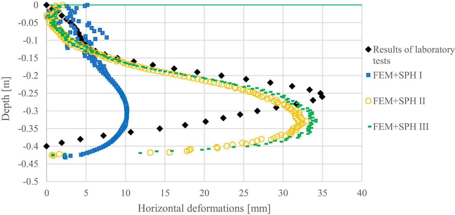
Figure 12

Source: Authors’ contribution.

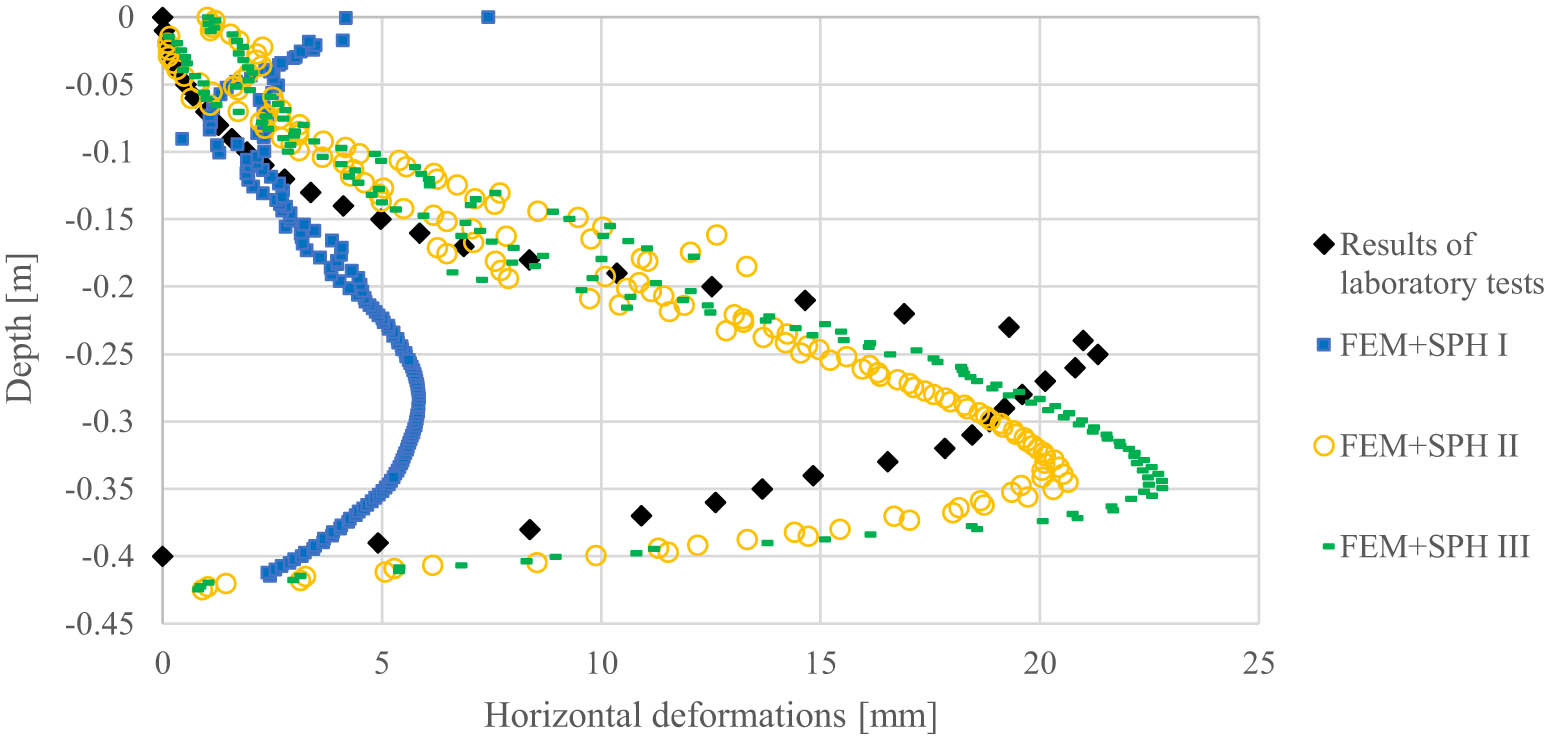
Figure 13

Source: Authors’ contribution.

4. Summary and conclusions

Enlarging the zone with SPH elements (from R _SPH/R _kmax = 1.6 to 3.5) allowed to reflect the entire process of forming the column. On the other hand, modelling the softening of the improved soil, observed during the driving of the column material in cohesive soils, allowed for the introduction of the aggregate into the load-bearing layer and obtaining a similar shape of the lower parts of the numerical columns to one of the columns from laboratory tests. The effect of modelling increasing the stiffness of the backfill as a result of the aggregates compaction is manifested in the shape of the propagation of the aggregate (semicircle). In the laboratory tests carried out, it was not possible to observe the displacements of the column material, but such observations were made by one of the authors of the article. The columns were formed in peat with a thickness of 0.5 m at a position that allowed the columns to be made and observed. The observed shapes of aggregate arrangement in individual discharges correspond (Figure 15) with the results of the FEM + SPH III model (Figures 9, 10b, d). The aforementioned observations confirm the authors of the article about the right direction to improve the model.

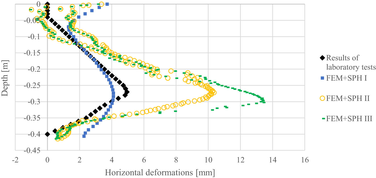
Figure 14

Source: Authors’ contribution.

Smaller volumes of columns, on the other hand, can be modified by increasing the volume of individual backfills. From Figure 7, it is clear that from the 10th of the pounder's discharge, the depths of the craters are greater than those recorded in laboratory studies. The use of the so-called small restart in the calculations means that before proceeding with the first discharge of the pounder, all the backfills must already be determined and entered into the model. The preliminary backfill heights were established based on the outcomes of the laboratory investigations. During the calibration of the numerical models, it was noted that, when simulating only the crater backfill, its height decreased by approximately 20–60%, which consequently increased the depth of the formed craters. This behaviour needs to be considered, necessitating an increase in the initial backfill height.

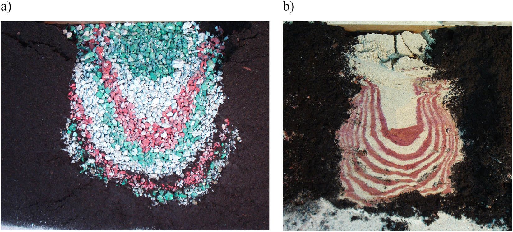
Figure 15

Source: Authors’ contribution.

The proposed models simulate lateral deformations in the immediate vicinity of the column quite well at a distance of 0.7–0.9 of the maximum diameter of the column. On the other hand, at a greater distance, they significantly overestimate them. Undoubtedly, the constitutive model used simulates the behaviour of the ground relatively well in the place of large displacements, as opposed to the area at a greater distance. It would be necessary to use more advanced constitutive models.

Funding information

Authors state no funding involved.

Author contributions

Sławomir Kwiecień: laboratory test, conceptualization and methodology, numerical calculation, writing – original draft preparation. Piotr Kanty: laboratory test, writing – review and editing. Ameen Topa: numerical calculation, writing – review and editing. Michał Sobota: numerical calculation, writing – review and editing.

Conflict of interest statement

Authors state no conflict of interest.