
1. Introduction
Determining the characteristic values of geotechnical parameters for separate lithological layers or otherwise defined soil zones is problematic across a number of applications [1–5]. These difficulties are mostly due to the natural variability of the soil, especially in transition zones surrounding the boundaries between distinct layers.
A geological/geotechnical model of the subsoil includes, among others, layers of soils and rocks with similar properties, defined using a number of criteria, including lithological (soils and rocks of the same type within a lithological series) and geotechnical ones (soils and rocks with similar strength, mechanical, and physical parameters) [2,5]. Consequently, layers defined in accordance with these criteria and adjacent to each other should be characterized by different values of certain basic geotechnical parameters. It can be assumed that in the central part of a single layer, these parameters are at a similar level, whereas in the transition zones at the boundaries of layers, there is a noticeable change in the values of certain parameters, including those not used for the layer definition.
In this study, the term ( transition zones ) refers to all zones in the vicinity of the estimated contact surface of layers in which significant variability of geotechnical and physical parameters occurs. For example, the transition zone between sandy and cohesive soils may consist of silty soils, sometimes referred to as transitional soils [6,7]. In this case, silty soils have significantly different values of certain geotechnical parameters than clayey and sandy soils. Such soils, in the area of normally consolidated soils, coincide with the soils described in the (Q t vs F r ) [8,9] nomogram as silt mixtures, clayey silt to silty clays.
The effect of spatial variability of soil properties applies to all research method, both the “classical” ones based on laboratory tests of soil samples and the one based on the results of field tests such as Cone Penetration Test with pore pressure measurement behind the tip called u 2 (CPTu), Flat Dilatometer Test (DMT), Seismic Cone Penetration Test (SCPT), or Dynamic Penetration Test (DPT).
The problem of determining layers based on CPTu soundings was discussed in the publication by Harder and von Bloh [10]. In this work, the authors signaled the possibility of using a simple mechanism consisting of determining the boundaries between layers based on the analysis of the dynamics of the increase in the values of cumulative curves and (original notation), where and is the distance between measurements.
According to Harder and von Bloh, the mechanism proposed by Harder and von Bloh [10] may hypothetically serve to identify transition zones between distinct lithological layers. Unfortunately, no detailed procedures for studying the dynamics of the function have been provided, and there are no clear criteria for defining the boundaries between “sublayers,” especially when the R f parameter is characterized by high variability or when it increases or decreases over a longer depth range. In such a situation, the shape of the curvature of the cumulative curve and the lack of straight sections do not allow for precise indication of the boundary points between the hypothetical layers.
If we understand the “dynamics” of the function I R ( z ) simply as the rate of change, such an examination will not provide any additional information due to the fact that examining the rate of change of cumulative curves I R ( z ) is equivalent to examining the first derivative of the function
where the first derivative is simply equal to the friction ratio R f (z).The function f ( z ) is a discontinuous function (which results from the way the parameter qc is measured during the static CPTu sounding), so it does not have a first derivative. In the abovementioned case, when the author writes about the first derivative, he means a continuous and differentiable function, e.g., a polynomial, passing through the points (z,f(z)) with an appropriate approximation.
Selected dispersion measures determined for the reference parameter X will serve as the basis for identifying the transition zones.
P.K. Robertson [6,11,12] pointed out a potential problem related to the analysis of CPTu soundings, concerning the influence of the cone indentation process on the readings of the q c parameter value as the cone passes through the boundaries of the sandy and cohesive zones. For this and other reasons, it is suggested [6] not to take such transition zones into account when interpreting geotechnical parameters. The distance from the layer boundary at which the effect of transition to another zone was observed depended on the type of soil on both sides of the boundary [11]. In most combinations, it was estimated at 3 ÷ 10 cone diameters, but for some configurations it exceeded 15 diameters.
As suggested by Robertson [6,12], the transition zones between adjacent soil layers can be determined based on the analysis of the variation in the parameter defined as the soil behavior type index I c , defined [7–9,13] as
where Q t is the normalized cone resistance and F r is the normalized local friction coefficient. The above parameter q t is the corrected cone resistance with respect to the pore pressure u 2 , and the parameter a is the so-called surface area factor.The study by Robertson [12] contains a general observation that the boundary between clay-like and sand-like soils occurs at values of I c ≃ 2.6. If the change in the I c value passes through this value and is characterized by high dynamics, then in such an area, a transition zone between cohesive and sandy soils should be expected.Robertson [12] raised the issue of interpreting CPT soundings in soil consisting of thin sand layers embedded in cohesive layers. In this study, a correction of q c using coefficients dependent on I c is proposed and empirical procedures (nomograms) for estimating these coefficients are given.
P.W. Mayne [14] observed the effects of increasing the cone resistance value q c in a clay layer when approaching a sandy layer and, similarly decreasing the q c value in a sandy layer when approaching a clay layer. The consequence of this is an incorrect estimation of soil parameters in thin layers and in transition zones between layers with strongly contrasting soil types. As a solution to this problem, Mayne cited [11,12] the estimation of the parameters of sandy zones by assuming an equivalent value of q t * (Figures 1 and 2) in these layers in accordance with the formula
where H A – the thickness of the sand layer, d c – the diameter of the measuring cone, q t – the corrected cone resistance determined in the central part of the sand layer, and K H – the correction factor.It should be noted that formula (7) was given in the study by Robertson [12,14] only for a thin sandy layer surrounded by cohesive layers. The symmetric situation, i.e., a cohesive layer surrounded by sandy layers, probably shows increased qt values according to Figure 1 (drawing on the right), but formula (7) cannot be applied in such a case.
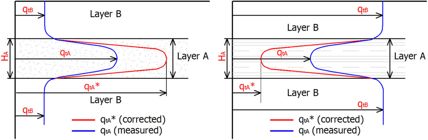
Figure 1
Correction qt in thin layers. Sand layer sandwiched between clay layers (left, quoted after [12,14]) and hypothetically symmetrically, a clay layer sandwiched between sandy layers (right). Formula (7) is defined only for the left-hand case.
Source: Author’s contribution.
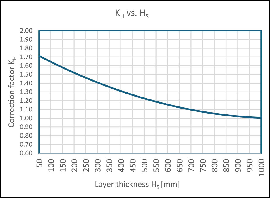
Figure 2
Correction factor (KH vs layer thickness HS) – (7).
Source: Author’s contribution.
Robertson [6,7] proposed to distinguish transitional soils , understood as soils in the zone between dilative and contractive soils, based on the nomogram (Q tn vs F r ). This nomogram uses the Soil Behavior Type Index I B [6,7] (Equation 10), different from the commonly used I c ).
It should be noted that the variability of the measured sounding parameter q c in the transition zone, near the boundary between different soil layers, is the sum of the variability resulting from the effect of the boundary between different soils on the q c reading and the natural variability of the soil properties in that vicinity, as described above. Currently, it is not possible to separate the independent effects of these factors on the variability of the sounding parameters.It can be assumed that the so-called boundary effect and/or thin layer effect reduce the dynamics of the rate of change of the q c parameter, while extending the depth range of this change, according to the scheme presented in Figure 3, but this hypothesis requires further in-depth research.
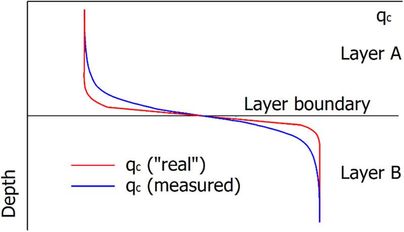
Figure 3
Hypothetical dynamics of q c change in the neighborhood of the boundary between layers.
Source: Author’s contribution.
The characteristic value X k of the geotechnical parameter X, according to Eurocode 7 (EC7) [15,16], is a conservative estimate of the value of this parameter in the context of the occurrence of a specific limit state.
EC7 allows to estimate the characteristic value of a geotechnical parameter through a number of methods, the most accurate of which is the assessment of the characteristic value based on a set of results of measurements of this parameter, which are then subjected to statistical analysis. Commonly used methods taken directly from EC7 and other methods based on the statistics σ (X) (population standard deviation) and s(X) (sample standard deviation) usually give an underestimated, sometimes unrealistic, value of the estimated parameter [4].
This is due to the high values of statistics σ(X) and s(X), which are a consequence of a number of random factors related to the research procedure and natural factors. The most significant factor influencing the values of σ(X) and s(X) is the natural spatial variability of the soil properties [1,4], particularly apparent in transition zones at the boundaries of separated layers and closely related to the genesis of the soils in these zones.
It should also be noted that the data we obtain from field investigations is often too sparse to generate meaningful statistics [3]. This observation is often described in the literature as the “curse of small sample size” [3].
2. Local measures of dispersion
The following statistical functions were adopted to analyze the course of variability of the reference parameter X.
2.1. Local mean value μ L(X(H))
Equation (11) defined for each depth H at which the parameter X is measured, as the mean value of parameter X calculated for all values of the reference parameter defined in the bilaterally closed depth interval <H − ΔH, H + ΔH>
where ΔH – the neighborhood radius for depth H, N – the number of measurements within the interval <H − ΔH, H + ΔH>, n – the index of subsequent measurements of parameter X within the interval <H − ΔH, H + ΔH>, and Xn – the values of parameter X within the interval <H − ΔH, H + ΔH>.2.2. Local standard deviation σL(X(H))
Equation (12) is defined for each depth H at which the parameter X is measured, as the standard deviation in the population calculated for all values of the reference parameter, defined in the bilaterally closed depth interval <H–ΔH, H + ΔH>
where the denotations are as defined above.2.3. Local coefficient of variation V L (X(H))
Equation (13) defined for each depth H as
3. Proposal for determining the vertical range of transition zones based on CPTu soundings
To estimate the extent of transition zones, it is proposed to use the cone resistance q c and the local measures of dispersion of this parameter’s values defined above – the Local Coefficient of Variation V L (X) (13) as a function μ L (X) (11) and σ L (X) (12) defined in Section 2.
In addition to q c , other sounding parameters, such as q t and I c , were considered in the initial phase of work in this study.
The u 2 values compared to the q c parameter are generally small [9], typically smaller by an order of magnitude. Therefore, considering the definition of the q t parameter, the difference between q t and q c values is very small, and their variability, measured, for example, using the local coefficient of variation, is practically identical. To test this thesis, q t calculations were performed for several dozen CPTu soundings, arbitrarily selected according to the negative criterion [Low q c values and high u 2 values] and compared with the q c values. The maximum differences between q c and q t reached 10–20%, but the dynamics of change (direction and rate of change) were practically identical. The zeros of the first derivative, indicating the location of the boundary between layers, were at exactly the same depth. In the vast majority of cases, the relative differences between q c and q t ranged from a few per mille to approximately 1%, so replacing q c with q t would practically not change or change only negligibly the transition zone ranges estimated using the method proposed in this study.
Using the I c parameter as a reference parameter is not a better solution than q c , but for different reasons. The values of this parameter usually range from 1 to 4, so their variability depending on soil type is relatively small (compared to the variability of q c ). Another argument is that I c is a parameter sensitive primarily to soil type, but even here, there are cases where I c cannot be used as the sole parameter to distinguish between clay and silt [17].
Other soil characteristics, such as compaction degree, plasticity degree, modulus, etc., are not closely correlated with I c . Therefore, assuming a broad definition of the transition zone as proposed in this study, the variability of I c does not allow for determining the existence and extent of such zones to a degree analogous to q c . Furthermore, according to the definition of I c (3), the variability of this parameter is decreased with increasing q c and f s due to the use of a logarithmic function in the definition. Therefore, for large values of q c and f s , determining the soil properties, the coefficient of variation of parameter I c shows relatively small variability.
CPTu static sounding – performed using a piezocone measuring the cone resistance q c , local friction on the sleeve f s , and pore pressure u 2 – is a research method well-suited for examining the characteristics of all types of soils with grain sizes ranging from clays to sands [8]. A number of soil parameters are moderately-to-highly correlated with the sounding parameters, including soil characteristics [8] such as soil type and layering, as well as parameters such as the relative density I D , the angle of internal friction Φ′, the undrained shear strength s u , the oedometric compressibility modulus M 0 , the shear modulus G 0 , the consolidation coefficient c, the preconsolidation coefficient OCR [18], and the cyclic resistance ratio CRR [12].
The correlation equations relating CPTu parameters to geotechnical ones largely include the parameter q c . They are not always applicable across all the site locations, but it can be assumed that at each location, the variability of q c is the result of the variability in a number of soil characteristics. Consequently, the identification of zones with high variability of q c , correlated with the values of basic soil parameters, also indicates zones with high variability of the values of these geotechnical parameters, and therefore – in accordance with the description of the transition zone given in Section 1 – transition zones.
Analysis of numerous CPTu soundings and boreholes near which CPTu soundings were performed demonstrated that in the vicinity of contact zones between distinct lithological layers, the values of the V L (X) and μ L (X) statistics calculated for the sounding parameters q c and f s increase significantly, reaching local maxima in close proximity to the hypothetical contact surface of these layers.
This effect is particularly visible for the parameter q c . For contact between layers with significantly different grain size compositions, the values of these statistics reach relatively high values at their peaks, while for layers with similar grain size, the peak values of these statistics are lower.
CPTu soundings performed by different operators using different measurement equipment with a resolution of 1 cm and 2 cm were analyzed. There was no noticeable effect of CPTu measurement resolution on the variability of the scattering measures σ L (X) and V L (X).
The proposed algorithm for estimating the extent of transition zones involves determining depth ranges in the vicinity of contact zones between distinct soil layers where the value of the statistics V L (X) ≥ A, where A is the critical permissible value of the coefficient of variation V L (X) and X is the reference parameter chosen by the author – the q c parameter.
Based on the analysis of many CPTu soundings, the radius ΔH of the neighborhood of each depth H was assumed to be ΔH = 10 cm, and the critical permissible value A of the local coefficient of variation V L (X), above which the area at depth H was classified as belonging to the transition zone, was assumed to be A = 0.1.
It should be noted that the ambient radius value ΔH was selected based on the analysis of a series of tests. The optimal value of this radius should be the subject of further research. A relationship between the optimal ambient radius value and the test region cannot be ruled out.
For such values, the transition zones are, in most cases, well-defined, and their spatial extent seems to be appropriately determined. The value of A = 0.1 corresponds to the observations in the study by Pula [4], where the coefficients of variation do not exceed 10% for materials such as steel or concrete (homogenized materials in which there is no effect analogous to the natural variability of the soil), while for soils, the values of cohesion or shear strength have coefficients of variation of the order of several dozen percent. In the many CPTu soundings analyzed, in which the occurrence of relatively homogeneous layers of greater thickness, either cohesive or sandy was found, the coefficients of variation V L (q c ) in the central part of these layers usually oscillate around several percent; on the other hand, the zones in which V L (q c ) have significantly higher values are also characterized by increased variability of the remaining sounding parameters f s and u 2 , which suggests a high variability of the soil properties within the defined layer or the presence of “sublayers” with slightly different properties than the rest of the layer.
Reducing the critical value of A results in an expansion of the transition zone, which in some cases is excessive and extends too deeply into the layer. In some instances, the local standard deviation estimated in the heterogeneous zones within the isolated layer was comparable to the local standard deviation in the transition zones near the layer boundary. In other instances, especially in cohesive soils, where the local mean value of q c is low and the measurement error of this parameter is relatively high, the local coefficient of variation V L (X) assumes relatively high values throughout the layer, and the identification of transition zones becomes impossible when the critical value of A is too low.
Adopting a critical value of A that is too high entails problems with delineating transition zones in the contact zones of soil layers with similar properties, in particular with similar grain size, because in the transition zones, such high values of V L (X) may not be achieved.
Figures 4 and 5 present the result of calculations of the local coefficient of variation V L (X) (8) (black graph illustrates the V L (q c ) parameter, described in Figures 4 and 5 as CVqc parameter) with parameters ΔH = 10 cm and A = 0.1, and the estimated transition zones, marked with a vertical red line next to the lithological profile. The profile on Figure 4 is interpreted from CPTu sounding using the Robertson ‘90 method [9], and the profile on Figure 5 comes from the profile obtained from the description of the borehole [19] next to which CPTu sounding was performed. The gray background in the q c graph indicates zones in which V L (qc) ≥ 0.1
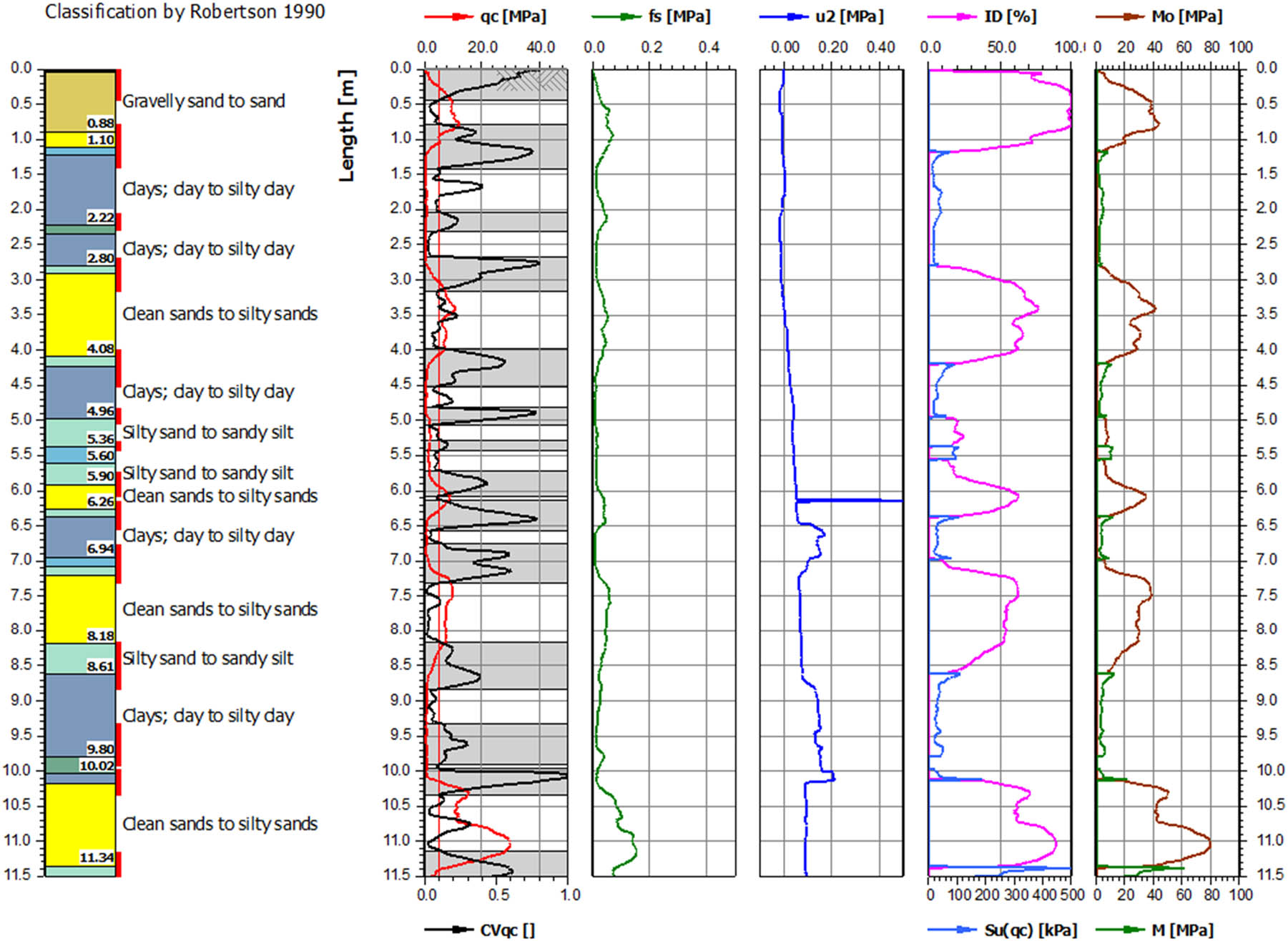
Figure 4
Hole E1. Determination of transition zones based on CPT soundings. The black plot next to q c , named on graph as CVqc, is the local coefficient of variation V L (X) (13) of the q c parameter. Gray background indicates transition zones. Classification by Robertson 1990.
Source: Author’s contribution.
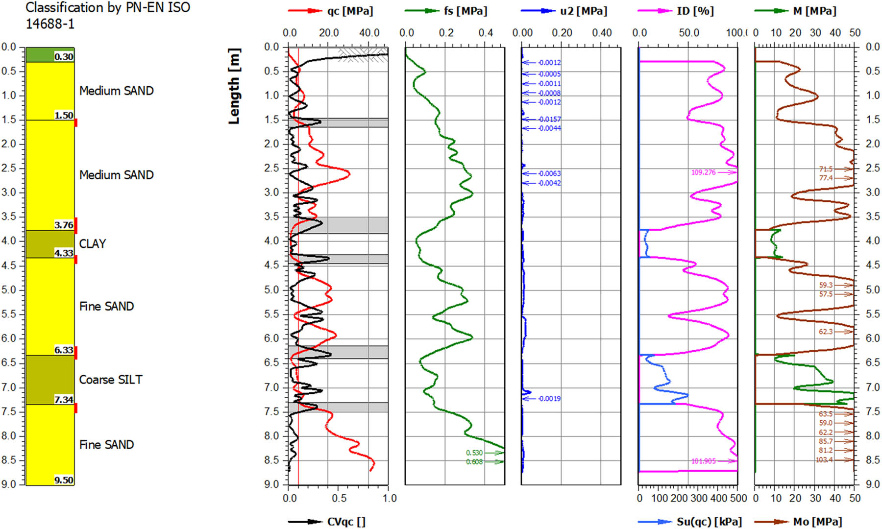
Figure 5
Hole E2. Determination of transition zones based on CPT soundings. The black plot next to qc, named on graph as CVqc, is the local coefficient of variation VL(X) (13) of the qc parameter. Gray background indicates transition zones. Classification by PN-EN ISO 14688-1:2018 [19].
Source: GEOdev Patryk Karolczyk.
4. Estimation of characteristic parameter values in selected soil layers or zones using statistical methods
According to EC7, the characteristic value X k of a parameter [1,5,15,16,20] X with a normal distribution with a mean μ and standard deviation σ should be determined as the 5 or 95% quantile of the probability distribution of this parameter. Depending on the parameter and the issue, a safer value is assumed.
In addition to the proposal included in EC7, there are a number of other methods for estimating characteristic values in the literature and in engineering practice, the common denominator of which is the use of formulas based on the following statistics:▪ μ (X) – the expected value of variable X (mean value of variable X in population),
▪ σ (X) – the population standard deviation of variable X,
▪ or their estimators m(X) and s(X).
Examples of such methods include the following estimations:
According to Schneider’s method [20]: X k = (sample mean value ± half of the sample standard deviation)
According to Polish Norm PN-81/B-03020: X k = (sample mean value ± population standard deviation m(X) ± σ(X))
According to Duncan’s method [21]: Xk = (5% quantile of the probability distribution of the variable X = μ(X) ± 1.645σ(X)) where σ(X) is estimated (after [4]) as
Confidence interval limits (CIL) of variable μ(X) at the confidence level [0.9] (referring to the 5% quantile of the probability distribution of variable X mentioned in EC7), calculated based on the t-Student distribution of variable μ(X). Depending on the type of parameter, the characteristic value X k is assumed to be the lower or upper limit of the confidence interval
The use of each of the abovementioned methods is usually associated with substantial underestimation of the characteristic values of geotechnical parameters, usually resulting from the high values of the σ(X) and s(X) statistics, especially when the number of measurements of these parameters is small. This problem was reported, in previous literature, [e.g., 1,3,4,12,22]. It should be noted that in Duncan’s method (19), the value of σ(X) is estimated using the maximum value Xmax and the minimum value X min in a given layer, and since these extreme values usually concern the area adjacent to the layer boundary, the omission of transition zones in the estimate also affects the estimation of characteristic values.
The high value of σ(X) and s(X) statistics is influenced by a number of random factors, the most problematic of which is the natural spatial variability of the soil, which cannot be eliminated by adjusting the test procedures [4,8]. This variability of the soil properties is particularly prominent in the areas near the layer boundaries. Consequently, the influence of measurements from these zones on the values of the σ(X) and s(X) statistics calculated globally for the entire layer is excessive and, in many cases, leads to an incorrect assessment of the values of the characteristic parameters, usually to their significant underestimation.
Determining the extent of transition zones and estimating characteristic values for the areas beyond them is theoretically possible using classical methods, i.e., by individually examining the surroundings of each layer boundary and performing repeated analyses of multiple high-quality soil samples. In the engineering practice, this is not feasible due to the very high cost of collecting and testing soil samples, the almost always insufficient sample size, and the lack of generally accepted and universal criteria that can unambiguously identify the boundary between a designated layer and the transition zone at its boundaries.
This study proposes the use of the static sounding method (CPTu) and the analysis of the variability of the basic sounding parameter q c to determine the extent of transition zones. According to the author, using other field tests, such as DMT, DPT, or SCPT, is not recommended due to the very low resolutions of these test methods, understood as the distance between the measurement points of the parameter values, and/or due to averaging of the results over zones with sizes related to the method’s resolution.
An alternative solution to the problem of excessive underestimation of characteristic values of geotechnical parameters, resulting from high values of σ(X) and s(X) statistics in the transition zones, proposed by the author, is to restrict the zones for which characteristic values of parameters are calculated to the central part of the layers and to omit measurements in transition zones at the boundaries of layers in the calculations.
This approach naturally raises the question of characteristic values of parameters in transition zones, which is very complex and beyond the scope of this publication.
This mechanism corresponds to Robertson’s suggestion [6] not to take into account the zones surrounding the boundaries between layers when interpreting geotechnical parameters from CPTu soundings.
It is an open question whether to assign such a characteristic value of the parameter only to the central part of the layers or to extrapolate it to the entire layer. It seems that for thin layers, due to the so-called thin layer effect [6,11,14], the latter approach combined with the correction of the q c value in accordance with the study by Robertson [12] is appropriate, whereas for layers with greater thickness, exceeding several diameters of the measuring cone, the former approach is also possible.
5. Influence of transition zones on the estimation of characteristic values of geotechnical parameters based on Eurocode 7 and other methods based on σ(X) and s(X) statistics
According to the author, characteristic values of geotechnical parameters should, to the highest extent possible, reflect conservative but realistic soil parameter values. Underestimating characteristic values should not be considered a pragmatic, safety improvement measure, as this is the purpose of the material coefficients specified in EC7 and the safety coefficients specified in all types of design guidelines.
The influence of transition layers on the estimation of characteristic values of geotechnical parameters related to strength, in particular, the degree of compaction I D , shear strength s u , angle of internal friction Φ , cohesion c, and oedometric modulus M, is doubled in “strong” layers situated between “weak” layers. The values of these parameters in transition layers are usually lower, which reduces the mean value of parameters calculated in the entire layer. Furthermore, the values of the statistics σ(X) and s(X) are higher in those layers, which further reduces the values of the estimates of 5% quantile of variable X (14) and estimations (17) ÷ (20) (Section 4). This results in, among other things, substantial underestimation of the calculated characteristic values. Eliminating transition zones from the calculations will result in a more realistic estimation of characteristic values and, in most cases, will produce more realistic, usually higher, values of these parameters than those obtained through “standard” calculations that take into account the entire layer.
The situation is somewhat different in “weak” layers located between “strong” layers. In this case, the presence of transition zones increases the mean value of the q c parameter, concurrently with an increase in the σ(X) and s(X) statistics. The final effect of omitting transition zones in the estimates of characteristic parameter values is not as obvious as in the reverse situation, due to the opposing effects of changes in the mean value and the σ(X) and s(X) statistics.
6. Calculation examples
The statistical functions μ L (X), σ L (X), and V L (X) described above were used to determine the transition zones. All calculations and analyses of CPTu soundings, including statistical functions and transition zone estimation, were performed using the CPT-pro software [23].
ΔH = 10 cm was assumed as the surrounding radius, and A = 0.1 was assumed as the limiting permissible value A of the local coefficient of variation V L (X).
To analyze the effectiveness of the proposed method, CPTu soundings were selected that contained both sandy and cohesive layers. In borehole E1, the classification interpretation was made according to the method developed by Robertson and presented in previous studies [8,9]. In borehole E2, the division into layers was made mainly based on the drilling results and described in accordance with the PN-EN ISO 14688-1 standard [19].
The impact of the proposed method on the characteristic values of the parameters is illustrated using the following parameters as an example:
I D (relative density in sands) estimated according to the formula described in the study by Jamiolkowski [24]
S u (undrained shear strength) estimated according to the formula described in the study by Lunne et al. [8] (with Nk = 14)
M (constrained modulus in fine soils) estimated according to the formula described in the study by Kulhawy and Mayne [25]
M 0 (constrained modulus in coarse soils) estimated according to the formula described in the study by Lunne et al. [8,26]
Table 1
CPT test E1. General characteristics.
| Averaged borehole profile. 5 sandy layers and 5 cohesive layers | Average for the hole E1 | ||||
|---|---|---|---|---|---|
| Layer thickness (m) | Central zone thickness (m) | Transition zone thickness (m) | Share of central zones | Share of transition zones | |
| Coarse soils | 0.76 | 0.48 | 0.28 | 62.63% | 37.37% |
| Fine soils | 0.77 | 0.50 | 0.28 | 64.08% | 35.92% |
Source: Author’s contribution.
Table 2
CPT test E2. General characteristics.
| Averaged borehole profile. 4 sandy layers and 2 cohesive layers | Average for the hole E2 | ||||
|---|---|---|---|---|---|
| Layer thickness (m) | Central zone thickness (m) | Transition zone thickness (m) | Share of central zones | Share of transition zones | |
| Coarse soils | 1.91 | 1.65 | 0.26 | 86.61% | 13.39% |
| Fine soils | 0.79 | 0.67 | 0.12 | 84.81% | 15.19% |
Source: Author’s contribution.
Table 3
Hole E1. Relative changes in selected parameters after omitting transition zones
| Hole E1 | Parameters | Average values in the hole | Relative changes in selected parameters after excluding transition zones | |||||||
|---|---|---|---|---|---|---|---|---|---|---|
| Mean value μ | Std dev s | Pop dev σ | Coeff of var V | Value acc. EC7 μ-1.645σ | CIL m- | Value acc. to Duncan μ-1.645σ σ=⅙(Xmax-Xmin) | Value acc. to Schneider μ-s/2 | |||
| % | % | % | % | % | % | % | % | |||
| Coarse soils | Point resistance q c (MPa) | 6.42 | 9.11 | −29.69 | −30.33 | −33.05 | 81.35 | 14.46 | 34.00 | 18.33 |
| Sleeve friction resistance f s (MPa) | 0.03 | 15.41 | −50.37 | −50.37 | −49.82 | 254.75 | 20.99 | 46.25 | 29.42 | |
| Relative density I D (%) | 59.87 | 1.38 | −34.42 | −35.10 | −35.31 | 12.79 | 2.68 | 9.68 | 4.03 | |
| Constr. modulus M 0 (MPa) | 25.52 | 9.12 | −32.05 | −33.34 | −34.64 | 80.53 | 14.83 | 32.87 | 18.56 | |
| Fine soils | Point resistance q c (MPa) | 0.51 | −8.79 | −54.11 | −54.40 | −52.18 | 63.42 | −3.42 | 40.00 | 1.24 |
| Sleeve friction resistance f s (MPa) | 0.02 | −8.96 | −39.12 | −40.25 | −38.39 | 1.89 | −4.08 | 16.40 | −1.19 | |
| Relative density I D (%) | 30.15 | −10.62 | −53.72 | −54.36 | −51.46 | 120.79 | −3.95 | 64.67 | 1.94 | |
| Constr. modulus M 0 (MPa) | 3.57 | −9.88 | −54.58 | −55.26 | −51.64 | 108.76 | −4.01 | 56.95 | −0.49 | |
Source: Author’s contribution.
Table 4
Hole E2. Relative changes in selected parameters after omitting transition zones
| Hole E2 | Parameters | Average values in the hole | Relative changes in selected parameters after excluding transition zones | |||||||
|---|---|---|---|---|---|---|---|---|---|---|
| Mean value μ | Std dev s | Pop dev σ | Coeff of var V | Value acc. EC7 μ-1.645σ | CIL m- | Value acc. to Duncan μ-1.645σ σ=⅙(Xmax-Xmin) | Value acc. to Schneider μ-s/2 | |||
| % | % | % | % | % | % | % | % | |||
| Coarse soils | Point resistance q c (MPa) | 16.12 | 7.94 | −4.63 | −4.69 | −11.57 | 65.54 | 10.26 | 26.18 | 11.68 |
| Sleeve friction resistance f s (MPa) | 0.26 | 6.51 | −12.37 | −12.05 | −17.10 | 27.09 | 8.52 | 15.61 | 9.56 | |
| Relative density I D (%) | 78.98 | 3.66 | −16.37 | −16.41 | −19.22 | 12.75 | 5.01 | 12.46 | 5.70 | |
| Constr. modulus M 0 (MPa) | 48.98 | 6.48 | −7.76 | −7.53 | −13.20 | 27.52 | 8.44 | 19.65 | 9.45 | |
| Fine soils | Point resistance q c (MPa) | 3.09 | 1.30 | −13.63 | −13.58 | −14.95 | 16.39 | 2.71 | 6.82 | 3.51 |
| Local friction resistance f s (MPa) | 0.10 | −1.47 | −16.84 | −15.46 | −15.44 | 5.49 | −0.47 | 4.76 | −0.52 | |
| Undrained shear strength S u (MPa) | 99.30 | 1.23 | −13.70 | −13.92 | −15.11 | 17.85 | 2.76 | 7.20 | 3.56 | |
| Constr. modulusM (MPa) | 24.57 | 1.29 | −14.83 | −12.75 | −15.28 | 18.29 | 2.73 | 7.01 | 3.91 | |
Source: Author’s contribution.
Preliminary analysis of the results indicates that omitting the transition zones has a significant impact on the basic parameter q c and the obtained values of characteristic parameters.
In borehole E1 (Figure 4, Tables 1 and 3), the mean values of q c in sandy soils increased on average by 9.1% and the values of the dispersion measures s, σ, and V of the q c parameter decreased by −29.7, −30.3, and −33.1%, respectively. At the same time, the characteristic values of selected geotechnical parameters increased significantly (2.7–80.5%) (Table 3).
In cohesive soils, the mean q c values decreased on average by 8.8%, while the characteristic values, depending on the estimation method, underwent significantly different directional changes – e.g., the undrained shear strength S u estimated according to EC7 increased by 120.8%, but according to the method based on determining CIL decreased by −3.9%. Such a large discrepancy results mainly from the change in the standard deviations σ and s (−54.4 and −52.2%, respectively) and from the influence of statistical coefficients (1.645 vs 0.342) in Equations (14) and (20).
Large increases in the values of the characteristic parameters S u and M were recorded in the Duncan estimate, by 64.7 and 56.9%, respectively. These arose due to the X max values being in the transition zone. Consequently, the estimated standard deviation ≅ decreased significantly, but these increases were still significantly smaller than in the estimate (14) (5% quantile).
In borehole E2 (Figure 5, Tables 2 and 4), the observed parameter value increases in sandy soils were lower than in the borehole E1 (up to several %), but still had a significant impact on the characteristic values of the parameters. For example, the value of undrained shear strength S u increased by 17.8% according to EC7 and by 2.8% according to CIL.
In cohesive soils in borehole E2, an increase in the obtained characteristic values was also observed – on average by several to a dozen or so percent.
When comparing boreholes E1 and E2, it should be noted that borehole E1 contains layers with an average thickness less than twice that of borehole E2, which translates into an increased proportion of transition zones (excluded from the calculations) in individual layers. Regardless of the differences between the boreholes, however, the basic conclusion is that transition zones are of fundamental importance for the methods for estimating characteristic values of geotechnical parameters based on σ and s statistics, even if their thickness is on the order of several to several dozen cm and they constitute several percent of the entire layer.
An important conclusion arising from the analysis of the results of calculations of characteristic parameter values is the high sensitivity of these values to the location of the estimated boundary between layers. A small change in the estimated location of this boundary causes significant changes in the extents of transition zones in adjacent layers, consequently changing the values of the μ, m, σ, and s statistics, and ultimately leading to significant changes in the values of the characteristic parameters.
7. Summary and conclusion
CPTu method is very sensitive to changes in soil properties. The main sounding parameter, cone resistance q c , is characterized by very high variability, which is closely related to the variability of the soil’s geotechnical parameters. Consequently, examining the variability of the q c parameter enables identification of zones where the variability of this parameter is high, indicating high variability of the soil properties.
The variability of the q c parameter is well-described by the local coefficient of variation V L (X), which is a function of the local mean value μ L (X) and the local standard deviation σ L (X).
Based on the examples of numerous CPTu soundings and boreholes near which CPTu tests were performed, it was found that in the vicinity of contact zones between distinct lithological layers, the values of the μ L (X) and σ L (X) statistics calculated for the q c parameter increase significantly and reach local maxima in close proximity to the contact surface.
The proposed algorithm for determining the extent of transition zones, which involves determining the depth ranges where the value of the local coefficient of variation of the parameter q c exceeds a given critical value A, appears to be effective in detecting the presence of transition zones and estimating their extent. The effectiveness of this method is high for adjacent soils with significantly different properties, but decreases when the adjacent soils have similar properties.
The proposed method for determining the extent of transition zones has been successfully validated in terms of its effectiveness in identifying the zones characterized by high variability of the q c parameter, i.e., zones characterized by significant variability in soil properties. Unfortunately, it was not possible to examine soil properties based on laboratory tests in these zones and unequivocally classify them as transition zones. This issue requires further research and precise criteria for classifying the indicated soil as belonging to the transition zone or to one of the adjacent layers based on laboratory test results.
It cannot be ruled out a priori that for specific areas, the parameters defining the proposed method, i.e., the surrounding radius ΔH and the critical value A of the parameter V L (X), will better reflect the ranges of transition zones at values other than the proposed ΔH = 10 cm and A = 0.1. This potential limitation requires further research. In particular, different optimal values of the parameters ΔH and A (critical value V L (X)) can be expected when using a CPTu cone with a cross-sectional area of 15 cm2. This results from the effect of the layer boundary on the measured values of the parameter q c (in accordance with the observations discussed in previous literature [7,9,11,14] cited in Section 1).
The attached calculation examples demonstrate that transition zones have a significant impact on the estimation of characteristic values of geotechnical parameters, even in boreholes where they constitute several percent of the entire layer’s thickness. Their excessive influence on the characteristic values of parameters determined for lithological layers can be reduced by limiting the calculations to only the central parts of the layers and omitting the designated transition zones from the calculations. This procedure will lead to a more representative estimate of the characteristic values.
A consequence of using this approach is the lack of estimation of characteristic values, as well as other representative parameter values in the transition zones. It is certainly not possible to use methods based on σ and s statistics due to their high values in transition zones. This problem requires a global solution, both at the paradigm level and in the form of detailed algorithms.
An important conclusion drawn from the analysis of the calculated characteristic values of parameters is the significant impact the correct definition of the boundaries between layers has on these values. Incorrect assignment of a fragment of the transition zone to an adjacent layer can significantly affect the characteristic values of parameters estimated using statistical methods based on the μ, m, σ, and s statistics. Calculating characteristic values only in the central parts of layers, omitting transition zones, solves this problem and makes the characteristic values of parameters independent of the precision of determining the boundary between layers.
Special attention should be paid to transition zones defined by the q c parameter, which assumes very low values, below 0.5 MPa. Such values typically characterize cohesive soils with a plastic to fluid consistency. In such areas, the relative variability of the q c parameter is high, and this is additionally accompanied by a larger relative measurement error. This results from the general fact that measuring instruments at the periphery of their operating range have a larger relative measurement error than in the central range. Consequently, the V L (X) parameter may assume excessively high values in these areas, thus affecting the correct estimation of the transition zone range.
The use of the method presented above, which involves direct statistical analysis of native sounding parameters without taking into account the interpretation of these sounding results in terms of estimating geotechnical parameters, may have a much broader application in the description of a number of soil features, the description of which is beyond the scope of this article.
Acknowledgments
Author wishes to thank to Mr. Rafał Tarczyński, whose IT expertise enabled the incorporation of the computational procedures required for the subject of the article into the CPT-pro program.
Funding information
Author states no funding involved.
Author contributions
The content of the article, with the exception of information cited from the referenced literature, is the result of the author’s own work. All aspects of this paper, including method for determining the extent of transition zones, the application of mathematical tools, conceptualization, interpretation of CPT tests, software implementation and formal analysis represent the author’s contribution.
Conflict of interest statement
The author declares no conflict of interest.
Data availability statement
CPT sounding files with results of interpretation are available at the following link: https://api.geosoft.com.pl/wp-content/uploads/2025/10/e1e2.zip