Estimation of the stability of tailings dams based on genetic algorithm-supported calibration results and monitoring data

The primary objective of the inverse problem is to estimate the FOS of a tailings dam for which monitoring data are available. Because FOS values cannot be measured directly and are primarily determined through numerical simulations, the inverse problem consists in identifying the model parameters that ensure consistency between monitoring data and simulation outcomes. Specifically, these parameters correspond to the material properties of the subsoil, dykes, and tailings.

Let

• p ∈ P p{\mathbb{\in }}{\mathbb{P}} denote the vector of unknown model parameters to be estimated,

• F : P → S {\mathscr{F}}{\mathbb{:}}{\mathbb{P}}{\mathbb{\to }}{\mathbb{S}} be the forward operator representing the numerical model, which maps model parameters p p to simulated outputs s = F ( p ) s{\mathscr{=}}{\mathscr{F}}(p) ,

• m ∈ S m\in {\mathbb{S}} denote the vector of real-world observations or measurements.

The objective is to find the parameter vector p ˆ \hat{p} for which the simulated data F ( p ˆ ) {\mathscr{F}}{\mathscr{\left(}}\hat{p}) best matches the observed data m m . This is commonly framed as an optimization problem, where the objective function to be minimized quantifies the discrepancy between simulation results and measurements (1) p ˆ = arg min p ∈ P f ( F ( p ) , m ) , \hat{p}={\rm{\arg }}\mathop{\min }\limits_{p{\mathbb{\in }}{\mathbb{P}}}f({\mathscr{F}}(p),m), where f f is the objective function, p ˆ \hat{p} is the optimal set parameters, and p {p} is any candidate set of parameters within the parameter space.

The objective function is typically defined using standard error metrics such as the mean absolute error, mean squared error, or root mean squared error (RMSE). In this study, RMSE was employed. It was assumed that the observation vector m m consists of two types of monitoring data: surface displacements measured at the slope surface, and piezometric heads measured below the ground surface. To combine these heterogeneous data types, a weighted RMSE was utilized, yielding the following form of the objective function: (2) f = 1 n ∑ i = 1 n w i ( F ( p ) i − m i ) 2 , f=\frac{1}{n}\mathop{\sum }\limits_{i=1}^{n}{w}_{i}\sqrt{{({\mathscr{F}}{(p)}_{i}-{m}_{i})}^{2}}, where n n is the total number of measurements across all monitoring locations, w i {w}_{i} is the weight assigned to the ith observation, with displacement data assigned a weight of 1, whereas for piezometric measurements, the weights were selected according to the measurement ranges at each sensor in order to balance their quantitative contributions to the objective function.

In cases where the parameter vector p leads to non-convergent numerical calculations, a very large penalty value is assigned to f f . The objective function f f is hereafter referred to as the unfitness metric [19], where lower values correspond to more desirable model outcomes.

The genetic algorithm has repeatedly been used as a method to identify the values of material parameters that enable agreement between measurements and numerical model results [20–24]. The genetic algorithm, first introduced by Holland [25], belongs to the class of metaheuristic optimization algorithms [26] and uses a population of candidate solutions that evolves over successive iterations, similar to natural evolution. It employs crossover, which involves exchanging information between two solutions, and mutation, which introduces small changes into a solution, to explore new points in the search space. Further information on genetic algorithms can be found in articles by Whitley [27] and Herrera et al. [28].

In this study, the genetic algorithm is implemented using an initial population of 24 individuals, i.e. 24 candidate solutions. Each individual is represented as a sequence of search parameters corresponding to the material properties being optimized. Coding is required only when identifying hydraulic conductivity; in this case, the parameter values must be transformed (as illustrated in Figure 1) to ensure compatibility with the algorithm’s operations. For all other cases, parameter values are used directly without additional coding.

Figure 1

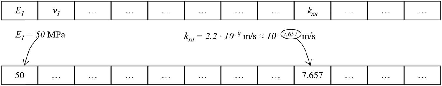
Solution coding into a sequence of real numbers.

In each iteration, the 12 worst-performing individuals are replaced by new ones, which are created by uniform crossover [29,30] (Figure 2) and mutation based on evolution strategies [31] and aggressive mutation [32]. During mutation, the value of each parameter is calculated according to x' = x·N(1, 0.05), where x′ is the parameter value after mutation, x is the parameter value before mutation, and N(1, 0.05) is a random number drawn from a normal distribution with mean value of 1 and standard deviation of 0.05.

Figure 2

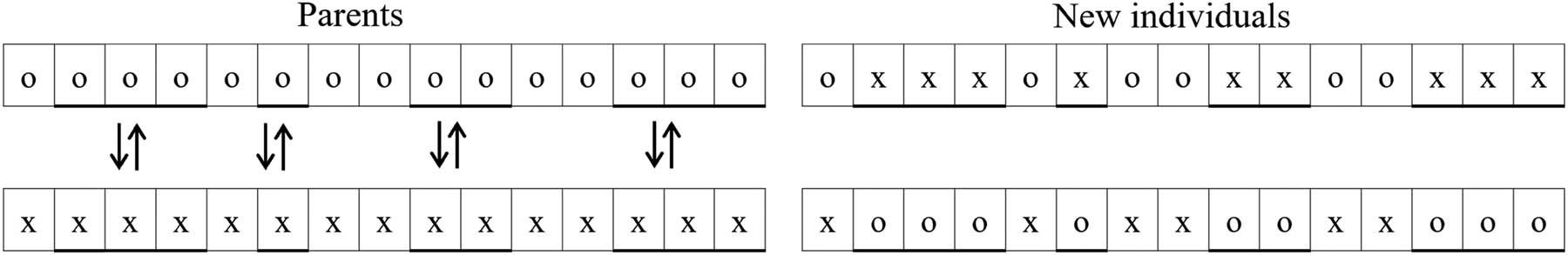
Uniform crossover.

The selection of individuals for crossover (i.e. parents) in the genetic algorithm is performed using a ranking-based approach [33]. In this method, individuals are ranked according to the value of the objective function, with better-performing individuals obtaining higher positions. The probability of an individual being chosen as a parent increases with its ranking position, ensuring that fitter individuals exert a greater influence on the next generation.

The identification algorithm itself was developed and implemented in Python [34], making use of the NumPy library for efficient numerical operations [35]. The custom script automates numerical simulations, processes output data, and quantifies unfitness (objective function value) for each individual, where each represents a numerical model defined by a specific set of material parameters. All key functions were coded independently by the author, which allowed for a customized genetic algorithm implementation, seamless integration of the script with the chosen numerical modelling software, and support for parallel execution of numerical simulations. This approach ensures both flexibility and computational efficiency in the parameter identification process. The algorithm was developed for the identification of typical soil parameters, including Young’s modulus, Poisson’s ratio, hydraulic conductivity, and strength parameters. Furthermore, it is possible to identify other parameters for more complex constitutive models.

During the minimization process using a genetic algorithm, numerous sets of parameters are evaluated over successive generations. From an optimization standpoint, only the best solution is typically of primary interest. However, all evaluated cases can provide valuable information about the numerical model and the relationships between parameters, as well as between parameters and outcomes. For example, if the genetic algorithm is initialized with a population of 24 individuals and generates 12 new individuals in each of 50 generations, more than 600 cases will be computed. This dataset can be analysed to derive additional insights. It should be noted, however, that many cases may be very similar, as the algorithm tends to converge towards an optimal or suboptimal (i.e. local) solution.

The objective is to identify relationships between calculated FOS values and the objective function. By analysing numerically generated data, as described above, it is possible to assess whether the calculated FOS values closely approximate the value obtained from the parameter set used to generate the monitoring data. This latter value is hereafter referred to as the True FOS. To examine these relationships, the Pearson correlation coefficient can be employed. Given two random variables, X and Y, the Pearson correlation coefficient, denoted as R X , Y {R}_{X,Y} , is defined as the covariance of X and Y normalized by the product of their standard deviations (3) R X , Y = cov ( X , Y ) σ X σ Y , {R}_{X,Y}=\frac{\mathrm{cov}(X,\hspace{0.25em}Y)}{{\sigma }_{X}{\sigma }_{Y}}, where cov ( X , Y ) \mathrm{cov}(X,{Y}) is the covariance of X and Y, σ X {\sigma }_{X} is the standard deviation of X, and σ Y {\sigma }_{Y} is the standard deviation of Y. The Pearson correlation coefficient ranges between −1 and 1. A value of zero indicates no linear relationship between the variables. A value of 1 signifies a perfect positive linear correlation, meaning that as X increases, Y increases proportionally. Conversely, a value of −1 indicates a perfect negative linear correlation, such that an increase in X corresponds to a proportional decrease in Y.

The interpretation of Pearson correlation coefficient values, according to Akoglu [36], is summarized in Table 1. This classification provides qualitative guidance for assessing the strength of linear relationships between variables based on the magnitude of the correlation coefficient.

Table 1

Correlation coefficient ( | R | |R| )	Strength of correlation
0.00–0.19	Very weak
0.20–0.39	Weak
0.40–0.59	Moderate
0.60–0.79	Strong
0.80–1.00	Very strong

Source: Author’s contribution.

If a significant linear correlation between unfitness and FOS is observed, it is reasonable to develop a linear regression model to describe their relationship. Such a model can be expressed as follows: (4) FOS = β 0 + β 1 × unfitness + ε , {\rm{FOS}}={\beta }_{0}+{\beta }_{1}\times {\rm{unfitness}}+\varepsilon , where β ₀ is the intercept, β ₁ is the slope coefficient representing the effect of unfitness on FOS, and ε is the error term. Importantly, the intercept β ₀ corresponds to the predicted FOS value when unfitness equals zero – that is, when there is no discrepancy between monitoring data and numerical model results. This prediction is particularly valuable in practical applications, as it provides an estimate of the FOS in situations where multiple FOS values remain equally plausible despite achieving minimal unfitness. Consequently, the regression model can serve as a useful tool for estimating FOS where direct evaluation is difficult. The simplicity and interpretability of the linear regression model make it a preferred starting point, compared to more complex models, particularly if linear association is confirmed. Moreover, this study investigates the relationship between the FOS and key material parameters to verify that hydraulic conductivity and shear strength, particularly the angle of internal friction, are critical for accurate FOS estimation in tailings dams.

The analysed tailings dam is based approximately on the Żelazny Most facility, as described by Skau et al. [9], Jamiolkowski [8], and Łydżba et al. [17]. The subsoil profile consists of three main stratigraphic units: Tertiary clays (hereafter designated as 1A), Tertiary sands (2B), and Quaternary sands (3C). The Tertiary clays represent the dominant layer, whereas the Quaternary sands are situated immediately beneath the ground surface. The Żelazny Most facility is a sequentially raised tailings dam constructed using the upstream method [37]. The rate of dam raising is approximately 1.25 m/year. Subsequent embankments are placed on previously deposited sediments, which exhibit finer grain sizes towards the centre of the reservoir.

The monitoring system at the Żelazny Most facility is described in detail by Stefanek et al. [37,38]. For the purposes of this study, it was assumed that the inverse problem uses data from six piezometers and three displacement gauges installed on the slope. A two-dimensional cross-section of the dam is considered, and the total number of measurement signals is 12, as each displacement gauge records both horizontal and vertical displacements.

The numerical model was developed using the FEM software ZSoil, assuming plane strain conditions. The discretization is shown in Figure 3. The model consisted of 4,765 quadrilateral enhanced assumed strain elements [39] and 12 triangular elements. Horizontal displacements were restrained on the vertical edges, while both vertical and horizontal displacements were blocked on the bottom edge. The initial state was determined only for the subsoil, which comprised three layers: 1A, 2B, and 3C, assuming a groundwater level at Y = 115 m. In this step, the analysis considered stationary groundwater flow and one-sided poro-mechanical coupling, i.e. the pressure distribution influenced the stress state. In subsequent stages, the construction of the dam was simulated by adding additional layers of elements, which were divided into three groups: dykes, beaches, and sediments, as proposed by Saad and Mitri [40]. A time-dependent pressure boundary condition, corresponding to the hydrostatic pressure distribution, was applied at the left edge of the model. Pressure boundary conditions were also applied to the bottom and top nodes of each newly added sediment layer. The values of these boundary conditions varied from the time the layer appeared until the next layer above was added, ranging from 0 to hγ and from −hγ to 0 for the bottom and top nodes, respectively, where h is the height of the layer and γ is the unit weight of water. Negative pressure indicates suction. During this period, the dry unit weights of dykes, beaches, and sediments increased from 0 to the target values presented in Table 2. This part of the analysis was carried out assuming full poro-mechanical coupling (i.e. the pressure distribution and stress state influenced each other), Darcy’s law, and the van Genuchten model [42]. An added layer height of 5 m, a rise rate of 1.25 m per year, a calculation time step of 0.25 years, and an analysis period from 1980 to 2020 were adopted.

Figure 3

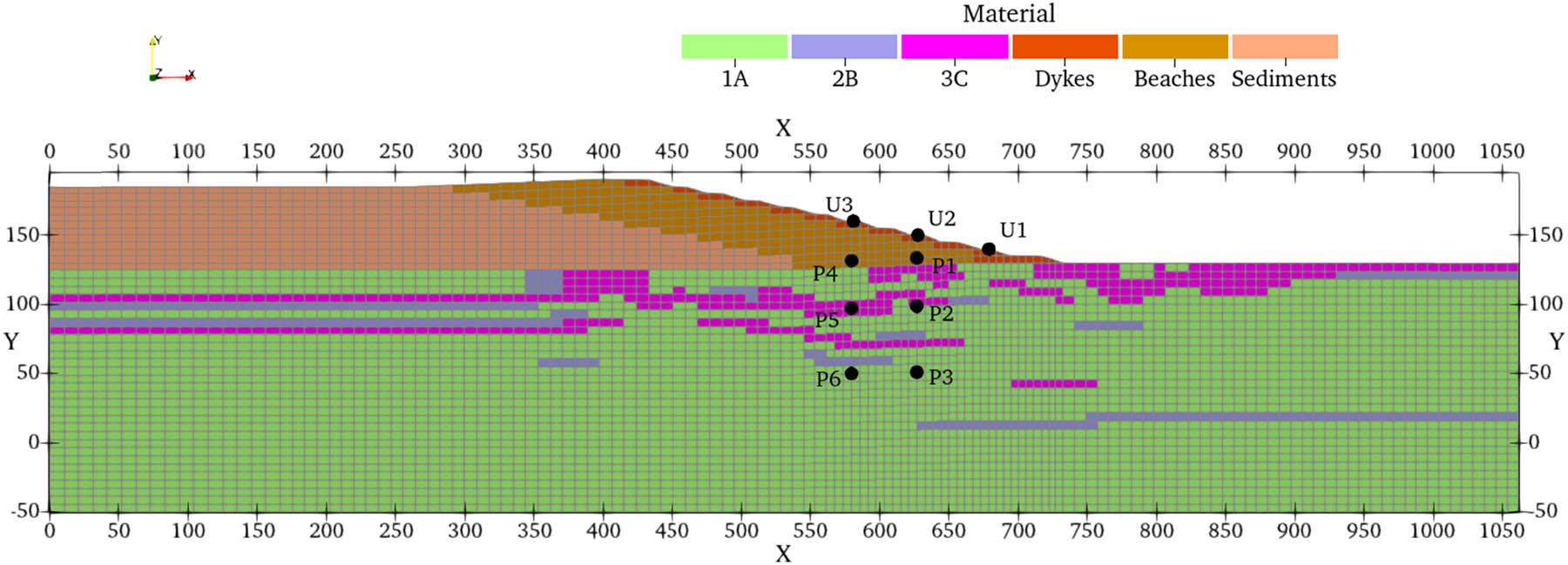
Numerical model and location of nodes selected as monitoring gauges.

Considering the origin and classification of the soils, it was determined that the subsoil layers 1A and 2B should be modelled using the Cap model. The Cap model incorporates two yield surfaces: a Drucker–Prager yield criterion and an elliptical cap, as illustrated in Figure 4.

Figure 4

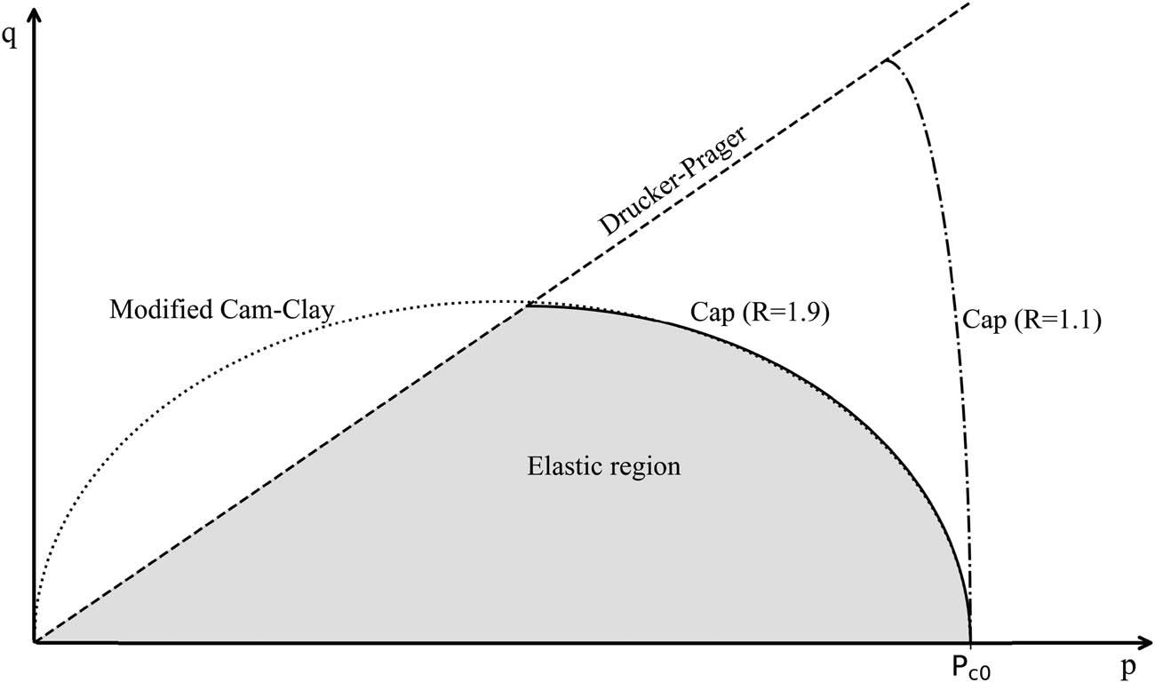
Cap model yield surface.

The cap yield surface is analogous to the Modified Cam-Clay model [43,44], developed to characterize the behaviour of cohesive soils, particularly clays. This surface constrains near-hydrostatic stress states, enabling the model to capture irreversible volumetric compaction – a key feature that makes it especially suitable for modelling clays and silty clays [45]. It is defined by two principal parameters: the preconsolidation pressure P _c0, which determines the intersection with the hydrostatic compression axis, and the shape parameter R, which characterizes the geometry of the elliptical cap. The preconsolidation pressure P _c0 represents the maximum historical isotropic effective stress experienced by the soil. The parameter R generally varies between 1.1 and 2.7, where the lower bound corresponds to a cap shape approaching a planar surface, and the upper bound corresponds to a more elliptical configuration. The evolution of the cap surface, commonly referred to as volumetric hardening, is governed by the parameter λ, which can be physically interpreted as the slope of the primary consolidation line in a semi-logarithmic e−log(p) space. Given the physical significance of P _c0 and λ, it is recommended that their values be obtained from laboratory tests [46]. The Drucker–Prager parameters are calculated automatically by ZSoil on the basis of angle of friction and cohesion, matching collapse load in plane strain with Mohr–Coulomb model for the same parameters [41]. When determining FOS using the strength reduction method, the cap surface is deactivated. Layer 1A was modelled with depth-dependent stiffness because of its substantial thickness. For elevations above Y = 110 m, Young’s modulus remains constant at the value shown in Table 2. Below this depth, it increases linearly achieving value multiplied by ME at Y = −50 m. The remaining materials were modelled using the Coulomb–Mohr model with the assumption of a non-associative plastic flow rule (including layers 1A and 2B) described by a dilatancy angle dependent on the angle of internal friction according to ψ = max(0.1φ, φ−25°).

As stated in the introduction, the use of synthetic (i.e. numerically generated) data is essential to verify whether a good fit to the monitoring data corresponds to an accurate estimation of the FOS values. Accordingly, three distinct parameter sets were selected to generate synthetic monitoring data. The parameter sets were selected to yield FOS values of 1.38, 1.48, and 1.64 (hereafter referred to as the true FOS values), corresponding respectively to a potential failure condition, a limit state, and a safe state. When effective strength parameters are employed in accordance with Polish legal regulations [18], the limit state corresponds to an FOS value of 1.5. The parameters for the three cases are presented in Table 2.

In Figure 3, the locations of the nodes used for data generation are shown. Three nodes were selected as surface displacement gauges (U1, U2, and U3), and six nodes were used to mimic piezometers (from P1 to P6). Illustrative examples of numerically generated monitoring data are presented in Figures 5 and 6.

Figure 5

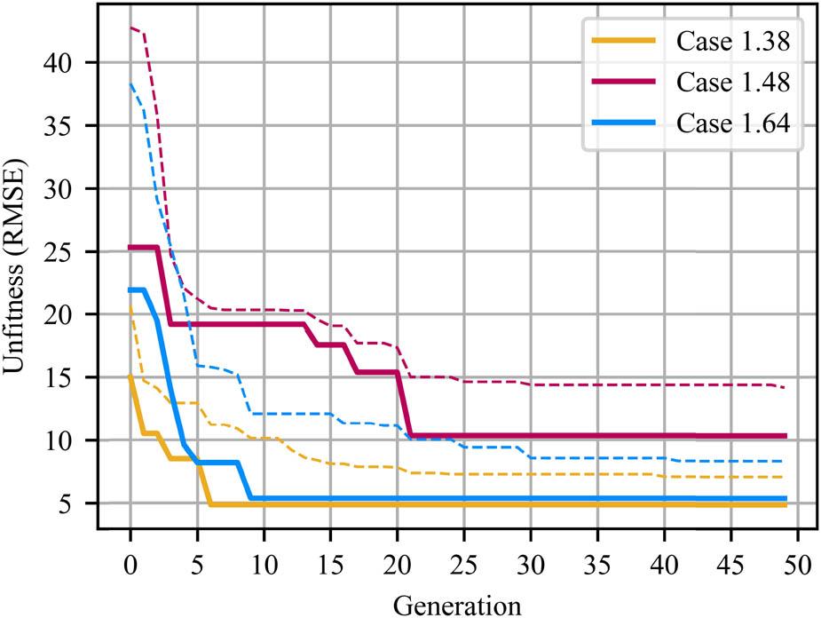
Unfitness and its mean (dashed) change during genetic algorithm calibration.

Figure 6

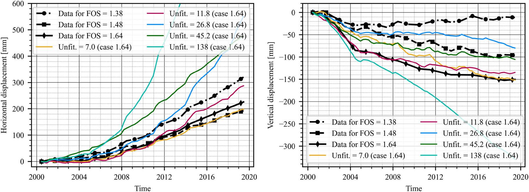
Match to horizontal (left) and vertical (right) displacement data of U2 gauge.

For each case, corresponding to a specific FOS value, the genetic algorithm calibration was performed three times. As previously described, the initial population consisted of 24 individuals, and at each iteration, the 12 individuals exhibiting the highest unfitness values were replaced with 12 newly generated individuals. The algorithm was terminated after 50 generations. The parameters being calibrated, along with their permissible ranges (i.e., the minimum and maximum values allowed during the genetic algorithm), are presented in Table 3. The boundary values were adopted based on experience from real-world applications; however, since a synthetic case is considered, the critical point is that the parameter values used to generate the monitoring data lie within the specified ranges. Parameters not subjected to calibration remained unchanged, with their values adopted as listed in Table 2. It should be noted that the hydraulic conductivity of the dykes was defined as dependent on the hydraulic conductivity of the beaches, according to a specified relationship (k _Dykes = 10k _Beaches) applied in both the horizontal and vertical directions. Additionally, the dilatancy angle was considered to be dependent on the angle of internal friction, as previously described.

Displacement values in the objective (unfitness) function are expressed in millimetres (mm), while piezometric heads are given in metres above sea level (m asl). A weighting factor of 10 was assigned to the piezometric measurements, based on empirical judgement derived from trial-and-error procedures and prior experience with real-world applications. Consequently, units for the unfitness metric are omitted in the following sections, as this quantity does not possess a direct physical meaning

Figure 5 shows how the unfitness of the best individual and the average of the six best individuals changed over successive iterations. Three cases out of nine were selected to illustrate both the best and worst calibration performance. In these cases, the value for the best individual stabilized before the 20th iteration, while the average value for the six best individuals continued to decrease after the 40th iteration.

Examples of the fit to synthetic monitoring data for various unfitness values in the case of FOS = 1.64 are presented in Figures 6 and 7. It is noteworthy that discernible differences are observed between unfitness values of 7.0 and 11.8, while the differences between 7.0 and 26.8 are substantial. Therefore, the fit corresponding to an unfitness value of 7.0 can be considered accurate, whereas unfitness values of 45.2 and 138 should be regarded as poor and inadequate, respectively.

Figure 7

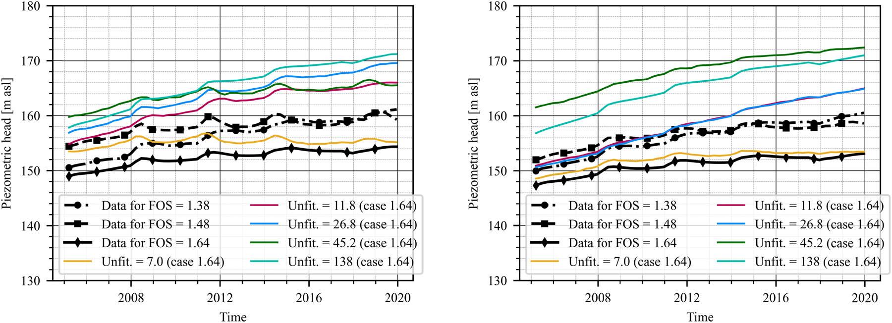
Match to piezometric data of P2 (left) and P3 (right) gauges.

First, the relationships between the FOS values and, respectively, hydraulic conductivities, angle of internal friction of the dominant layer 1A, and the value of the objective function were examined, as illustrated in Figure 8. The results from the three calibrations for each case were considered collectively. Blue dots indicate non-repeating individuals from the genetic algorithm calibrations, while the red dot represents the true values of the FOS and the relevant parameter. The findings indicate a moderate positive correlation (Pearson coefficient ≈ 0.5) between vertical hydraulic conductivity and FOS values. It is evident that higher FOS values are attainable only with higher vertical hydraulic conductivity. For higher values of the angle of internal friction, a similar, though less pronounced, relationship is observed. The FOS value is weakly correlated with horizontal hydraulic conductivity and unfitness. Notably, poor fits, defined as those with unfitness above 150, are predominantly associated with low FOS values (below 1.20), whereas good fits typically exhibit FOS values above 1.15. Most importantly, if only one of the three selected parameters is correctly reproduced (while the other two vary freely), the resulting FOS exhibits significant dispersion. This demonstrates that correct identification of a single parameter is insufficient. Consequently, FOS values were subsequently investigated under the assumption that the selected parameters were correctly identified. Values within the range of φ _true ± 0.5° (with φ _true denoting the angle of internal friction of 1A, as provided in Table 2) were considered to represent a correctly identified angle of internal friction, while for hydraulic conductivity, the ranges were assumed to be symmetrical with respect to the true value on a logarithmic scale, as illustrated in Figure 9.

Figure 8

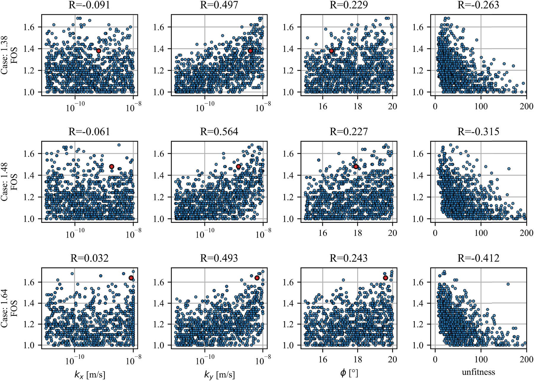
Relationships between FOS and parameters or unfitness; red dot indicates true values of FOS and parameters, and R is Pearson coefficient.

Figure 9

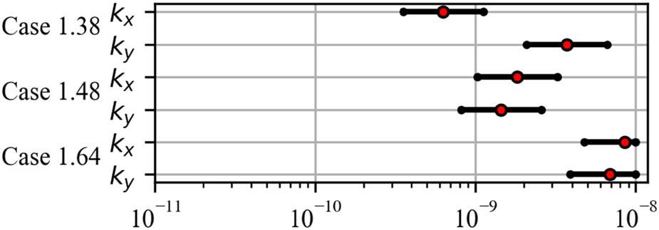
Hydraulic conductivity ranges assumed to be correct identification.

All cases with accurately identified hydraulic conductivity and angle of internal friction are presented in Figure 10. It can be observed that the number of such cases remains limited: five for case 1.38, three for case 1.48, and ten for case 1.64. The figure illustrates the relationship between unfitness and FOS. The wide range of unfitness values is expected, as displacement results contribute to unfitness and other parameters, primarily Young’s modulus, play a significant role. Importantly, the occurrence of inaccurately reproduced FOS values suggests that parameter identification is insufficient. The maximum differences between the true and calculated FOS values are 0.18, 0.48, and 0.60 for cases 1.38, 1.48, and 1.64, respectively.

Figure 10

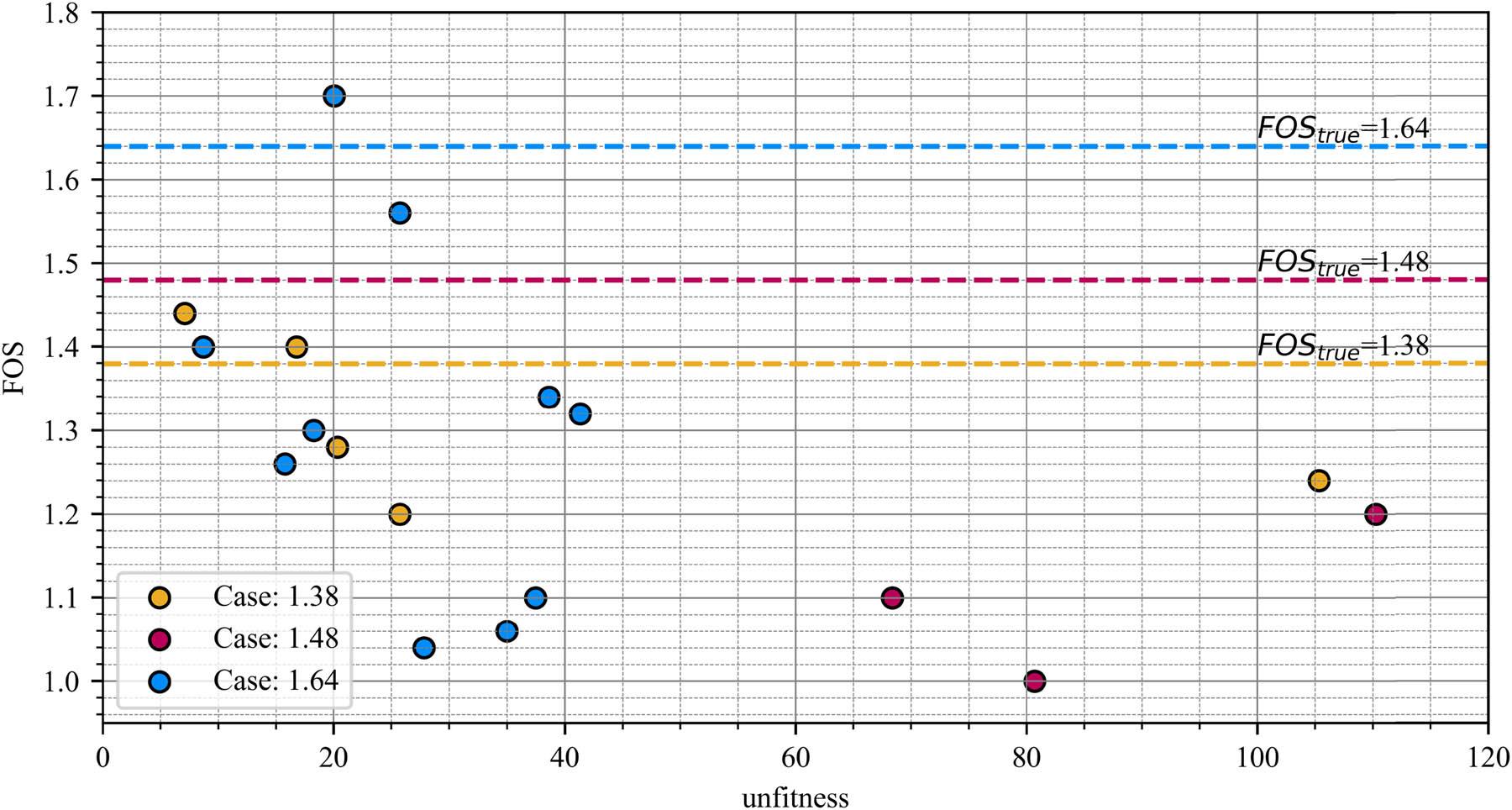
FOS values for correctly identified hydraulic conductivity and angle of internal friction.

In view of the findings and the aforementioned influence of the pore pressure distribution on the calculated FOS values, it was decided to investigate whether the accurate representation of piezometric measurements increases the likelihood of obtaining precise FOS values. Figures 11–13 illustrate the relationship between the FOS values and the RMSE calculated solely from piezometer data. In all three cases, the Pearson correlation coefficient was approximately below −0.70, indicating a strong negative correlation. A linear regression was used to formulate a simple model, and, assuming an RMSE of zero, meaning a perfect fit, the FOS values were estimated. Notably, FOS values calculated in this manner were close to 1.50 in each case. This outcome can be attributed to two principal reasons. First, the use of the same numerical model and identical parameter ranges in each of the three cases has a considerable impact. Second, the differences between the piezometric measurements for the three cases are not substantial, with average RMSEs around 5.0 (for comparisons of cases 1.64 vs 1.48 and 1.64 vs 1.38), or even 2.0 (for case 1.48 vs 1.38). Consequently, a satisfactory fit in one case is also likely to be satisfactory in the others. When calculated solely from piezometric data, the RMSE can be interpreted as the mean difference in metres per observation. Restricting the set to cases with a correctly identified angle of internal friction made it more likely to achieve accurate FOS values. Although the Pearson coefficients increased in these cases, the correlation should still be interpreted as previously discussed. Importantly, the estimated FOS values remained skewed towards 1.50.

Figure 11

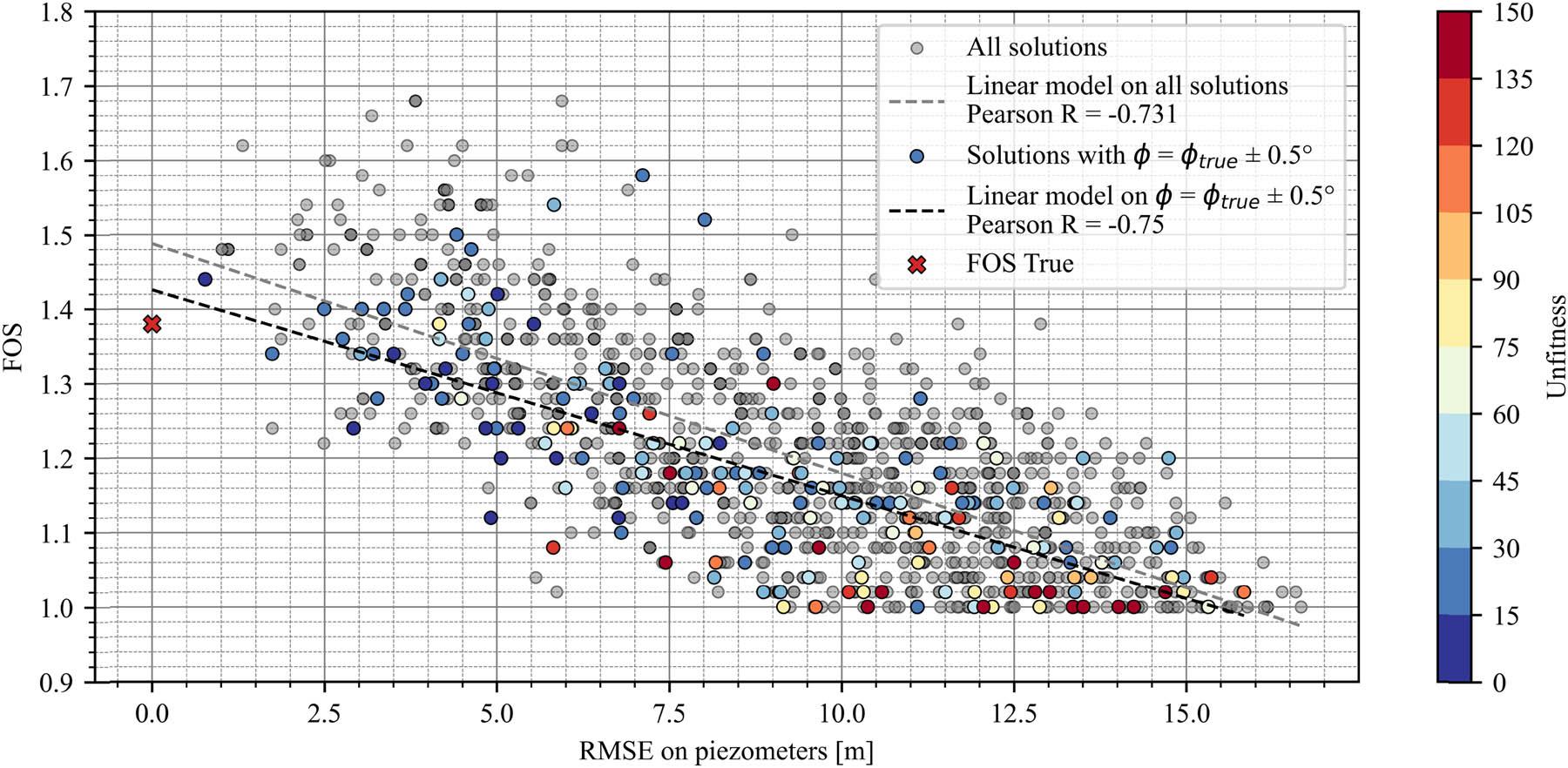
Relationship between piezometer fit (expressed as RMSE) and FOS in case 1.38.

Figure 12

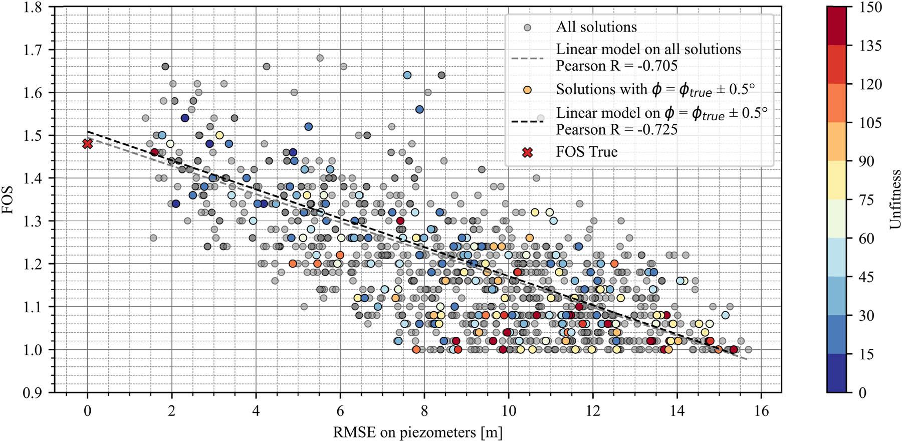
Relationship between piezometer fit (expressed as RMSE) and FOS in case 1.48.

Figure 13

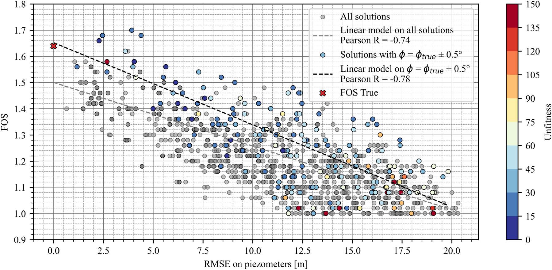
Relationship between piezometer fit (expressed as RMSE) and FOS in case 1.64.

It is important to consider the underlying reasons for the observed linear correlation. Assuming that lower pore pressure values correspond to higher FOS, it follows that cases characterized by low FOS and high RMSE represent situations where the numerical predictions substantially exceed the measured (or synthetic) piezometric data. Intuitively, low RMSE values should be associated with FOS estimates that closely approximate the true value. Therefore, it is plausible that Figures 11–13 exhibit a converging relationship between FOS and RMSE. However, there are few, if any, cases with both high RMSE and high FOS values exceeding the true value. This finding may be attributed to the imposed boundary conditions, particularly those concerning pressure, which are designed to simulate sediment deposition within the reservoir and the water level at the right boundary of the model. Given these boundary conditions and the dam’s geometry, achieving low pressure distributions is not feasible. Consequently, it can be concluded that the numerical model was appropriately constructed for the considered monitoring data.

The accuracy of FOS estimation was analysed by excluding the best individuals from the development of the linear regression model. Figure 14 presents plots of the FOS values obtained from the linear regression model, drawn exclusively for individuals with errors exceeding the values shown on the horizontal axis. The analysis focused on the case with a true FOS of 1.64 and considered two error metrics RMSE calculated solely from piezometric data, and unfitness. Three separate calibrations were distinguished, and their combined results were also shown. It is evident that in this case, the estimated FOS remains stable and close to the true value when the RMSE for piezometric data is below 5 or unfitness is below 25. The latter value corresponds to the best individual from the initial population in the worst case. When the results of all three calibrations are combined, a lower variance in FOS values is observed, with abrupt drops or increases eliminated. This confirms that multiple runs of the genetic algorithm can be advantageous, as different near-optimal solutions can be obtained using the same heuristic.

Figure 14

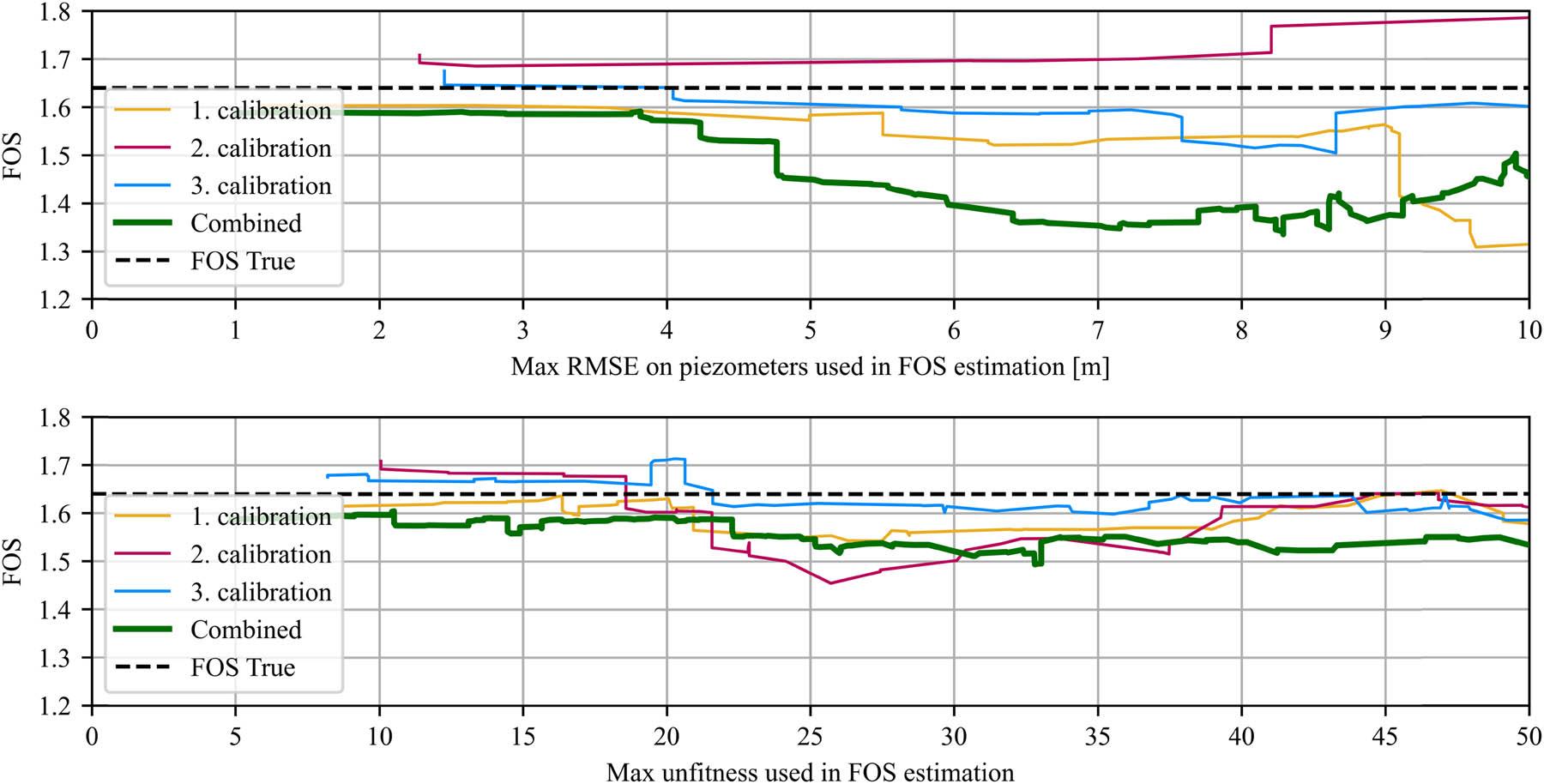
FOS estimated using individuals with value above RMSE calculated on piezometers (above) or unfitness (below).