
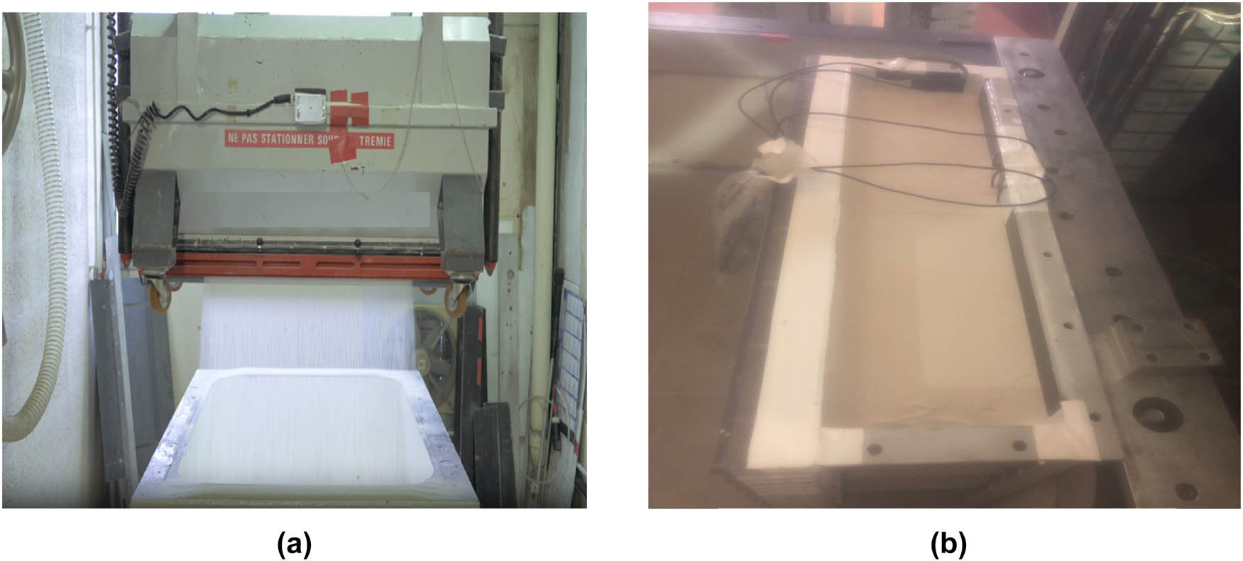
Figure 1
Sand preparation process: (a) sand raining technique and (b) prepared strongbox.
Source: Author’s contribution.
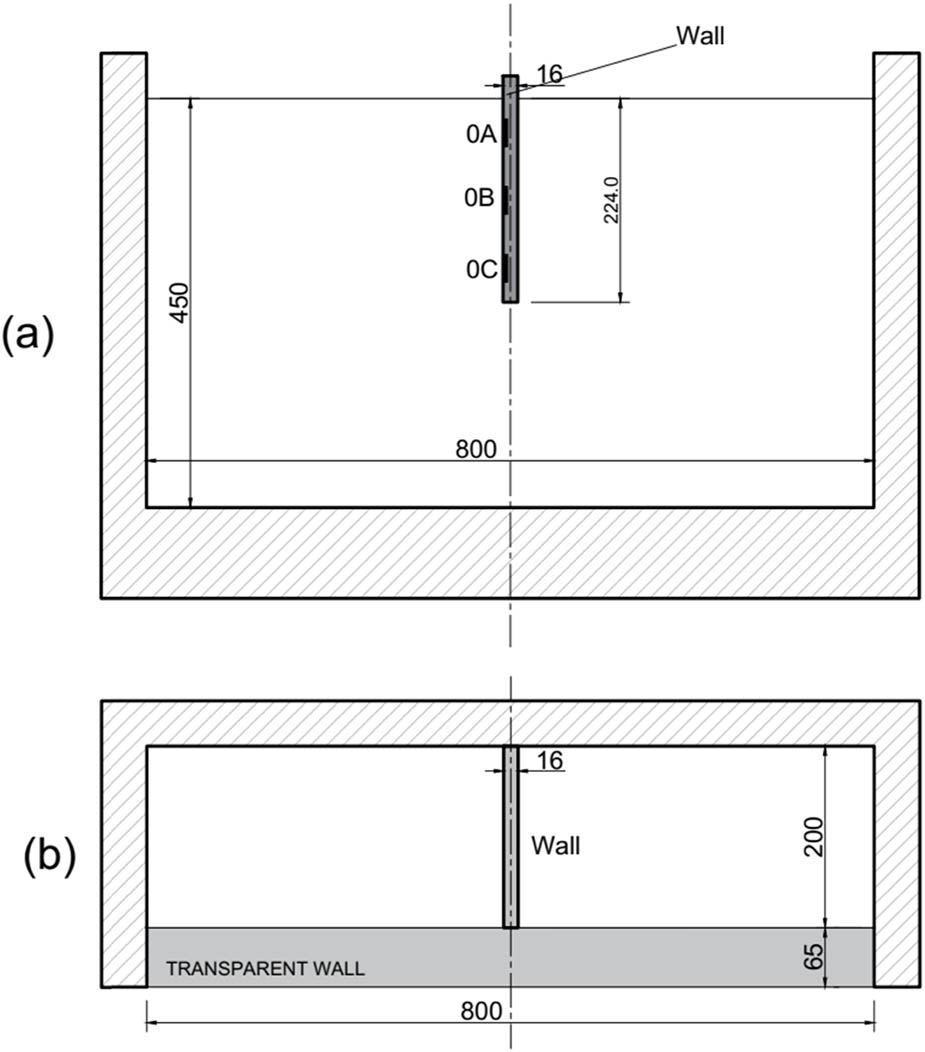
Figure 2
Experimental setup layout: (a) section view and (b) plan view at the end of wall installation. All dimensions in mm.
Source: Author’s contribution.
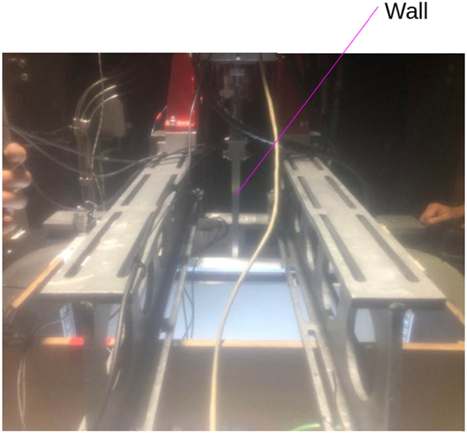
Figure 3
Experimental setup with model walls and loading frame configuration.
Source: Author’s contribution.
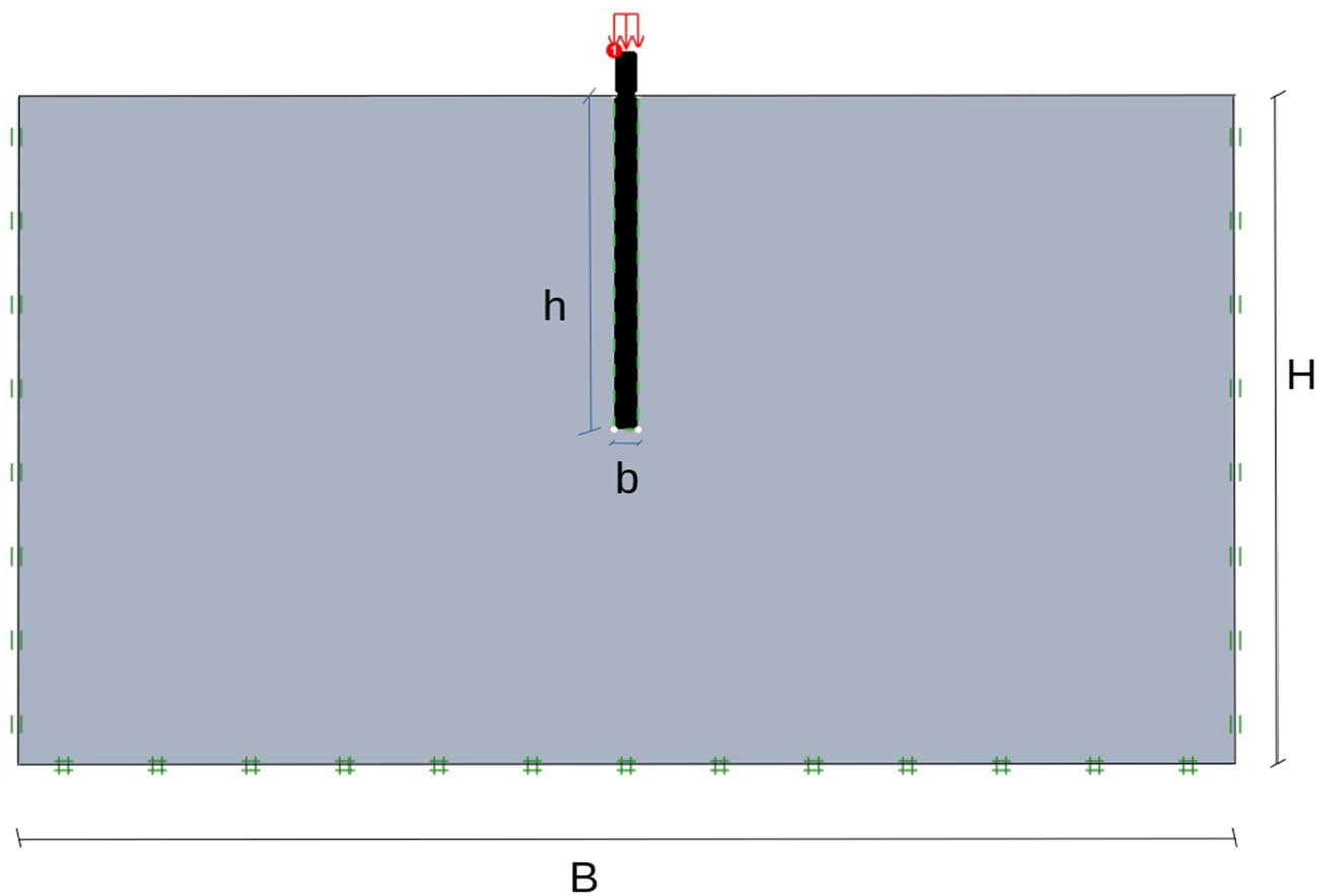
Figure 4
Numerical model setup in OPTUM G2.
Source: Author’s contribution.
Table 1
Properties of sand used in OPTUM G2 analysis [25].
| Property | MC model | HMC model |
|---|---|---|
| Young’s modulus (E) | 35 MPa | |
| Friction angle (φ′) | 31.5° | 31.5° |
| Cohesion (c′) | 0 | 0 |
| Poisson’s ratio (ν) | 0.3 | 0.3 |
| Unit weight (γ) | 16 kN/m3 | |
| Reference Young’s modulus (E 50,ref) | 40 MPa | |
| Unloading modulus (E ur,ref) | 75 MPa | |
| Earth pressure coefficient (K 0) | 0.47 | 0.47 |
| Dilatancy angle for non-associated flow (ψ) | 5.0° | 5.37° |
| Reference stress (p ref) | 100 kPa | |
| Hardening parameter (m) | 0.5 | |
Source: Author’s contribution.
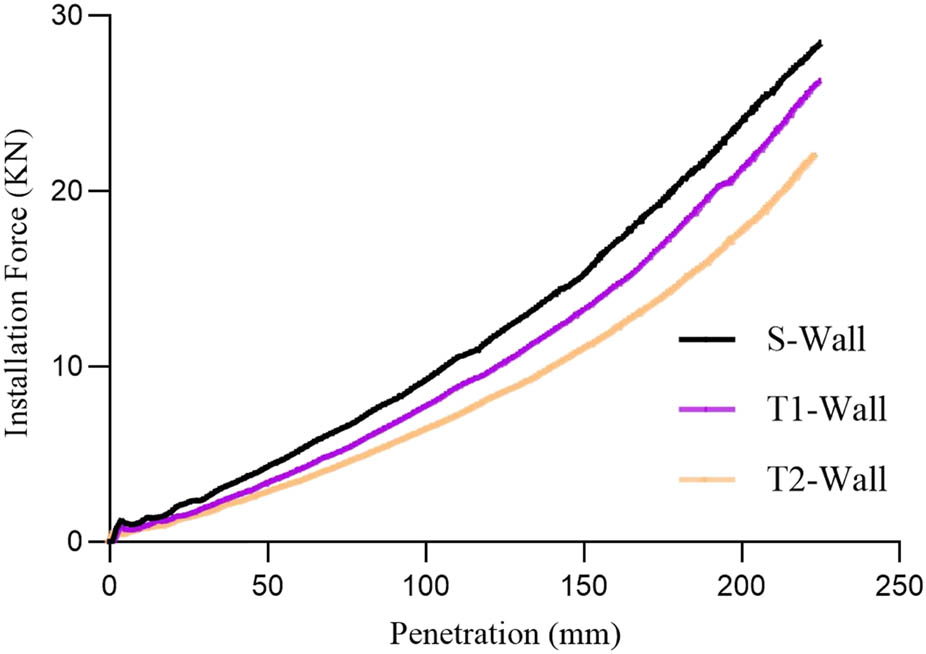
Figure 5
Load at pile head–displacement curves of walls from centrifuge experiments during the installation phase.
Source: Author’s contribution.
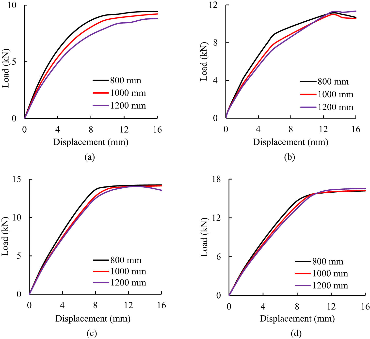
Figure 6
Effect of boundary conditions (container size) on the load–displacement curves: (a) HMC – lower bound, (b) HMC – upper bound, (c) MC – lower bound, and (d) MC – upper bound.
Source: Author’s contribution.
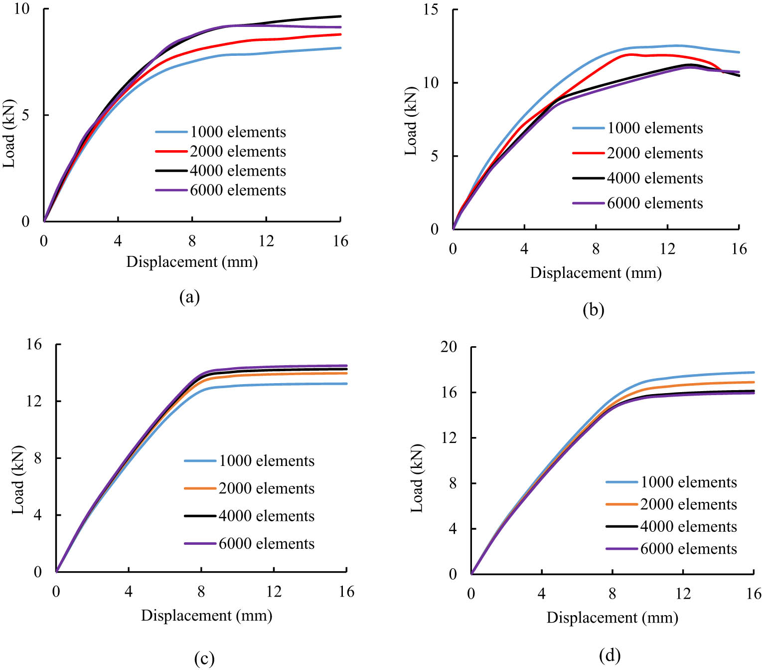
Figure 7
Effect of mesh density on load–displacement curves: (a) HMC – lower bound, (b) HMC – upper bound, (c) MC – lower bound, and (d) MC – upper bound.
Source: Author’s contribution.
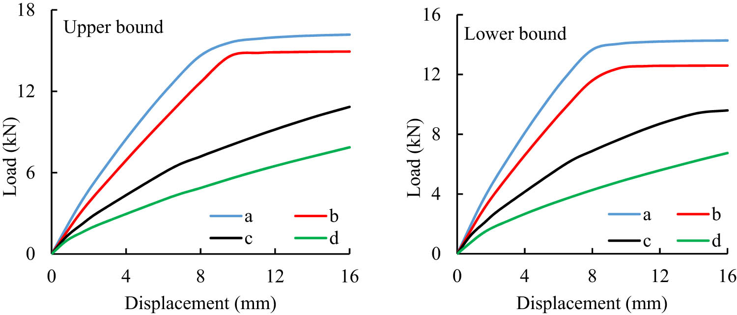
Figure 8
Load–displacement curves for different combinations of MC models with associated and non-associated flow rules.
Source: Author’s contribution.
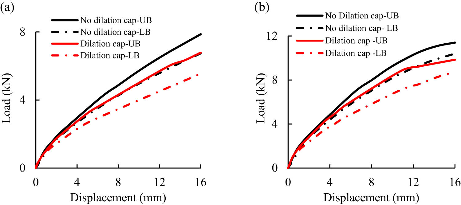
Figure 9
Effect of dilation cap on the load–settlement curves using (a) HMC model and (b) MC model.
Source: Author’s contribution.
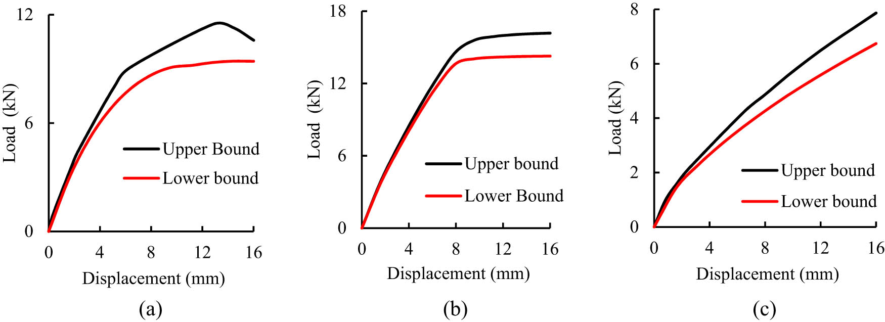
Figure 10
Load–displacement curves of the S wall using (a) HMC model, (b) associated MC model, and (c) non-associated MC model.
Source: Author’s contribution.
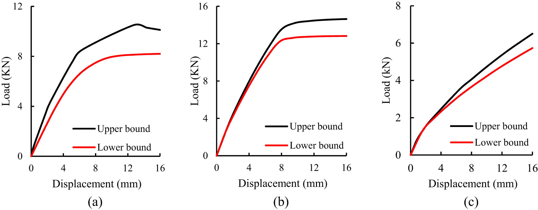
Figure 11
Load–displacement curves for the T1 wall using (a) HMC model, (b) associated MC model, and (c) non-associated MC model.
Source: Author’s contribution.
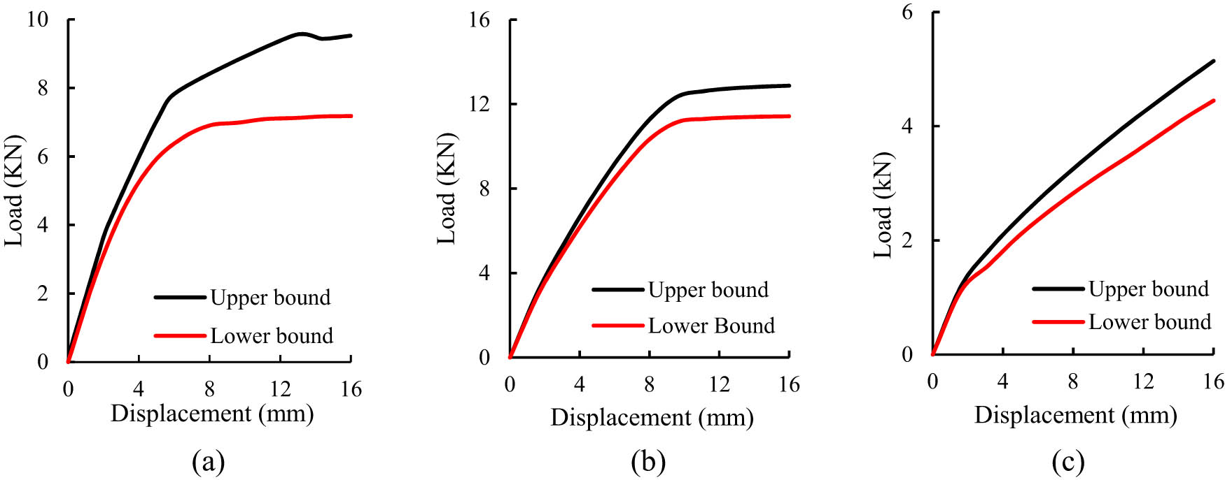
Figure 12
Load–displacement curves for the T2 wall using (a) HMC model, (b) associated MC model, and (c) non-associated MC model.
Source: Author’s contribution.
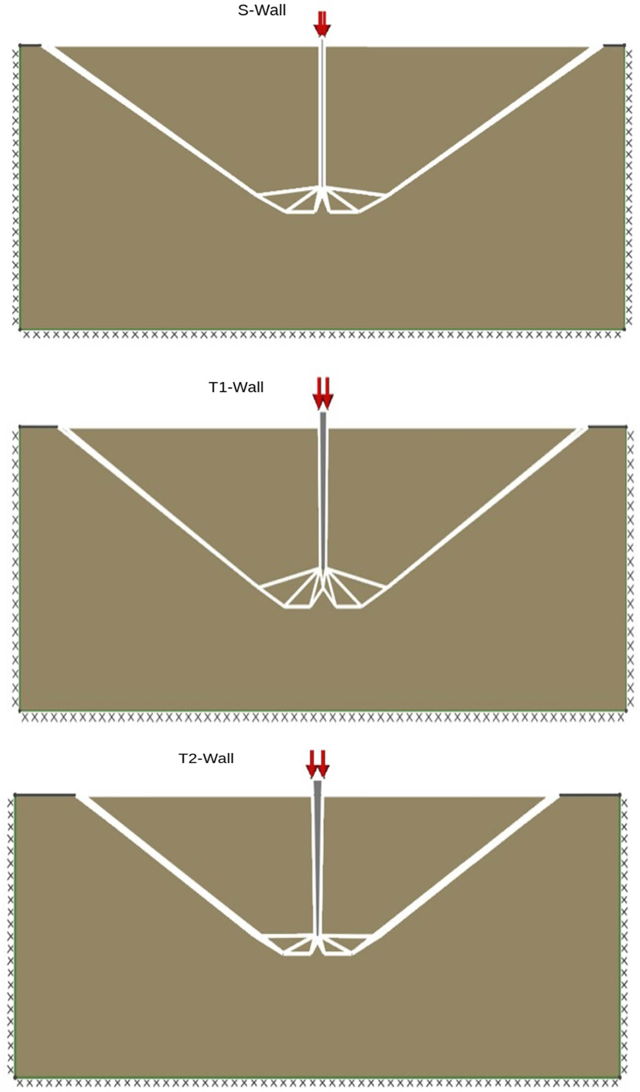
Figure 13
Failure mechanisms of the straight (S), moderately tapered (T1), and sharply tapered (T2) walls.
Source: Author’s contribution.
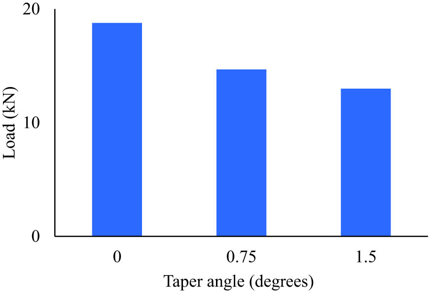
Figure 14
Failure load comparison for S, T1, and T2 walls at the end of installation.
Source: Author’s contribution.
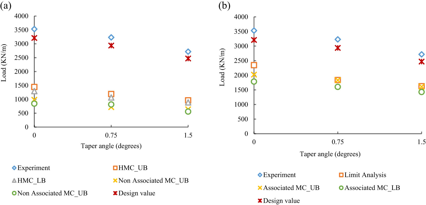
Figure 15
Comparison of numerical and experimental analysis (prototype scale) for (a) non-associated flow rule and (b) associated flow rule.
Source: Author’s contribution.
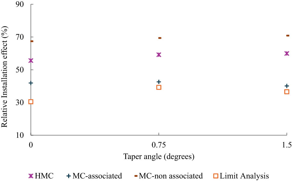
Figure 16
Relative installation effects (%) as a function of taper angle.
Source: Author’s contribution.