
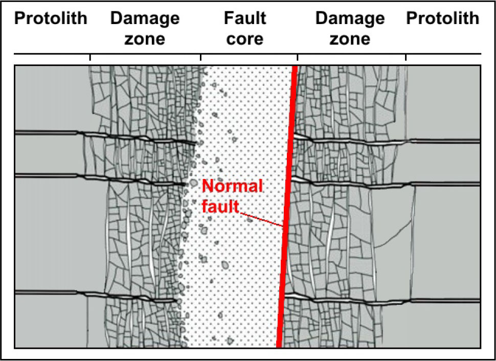
Figure 1:
Constitutive elements of a fault zone (from: [10] modified).
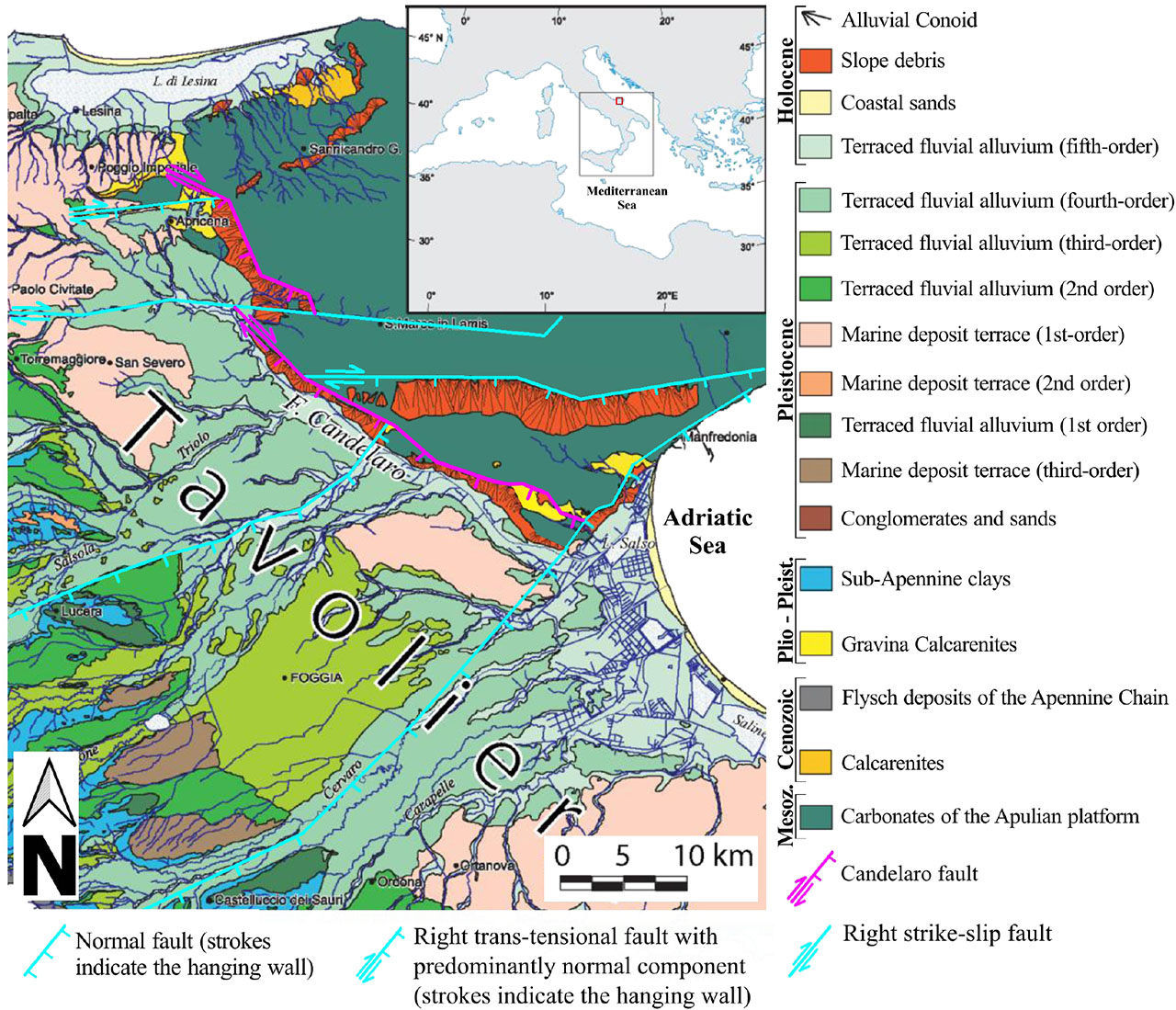
Figure 2:
Schematic geostructural map of the ‘Candelaro’ fault area (from: [27] modified).
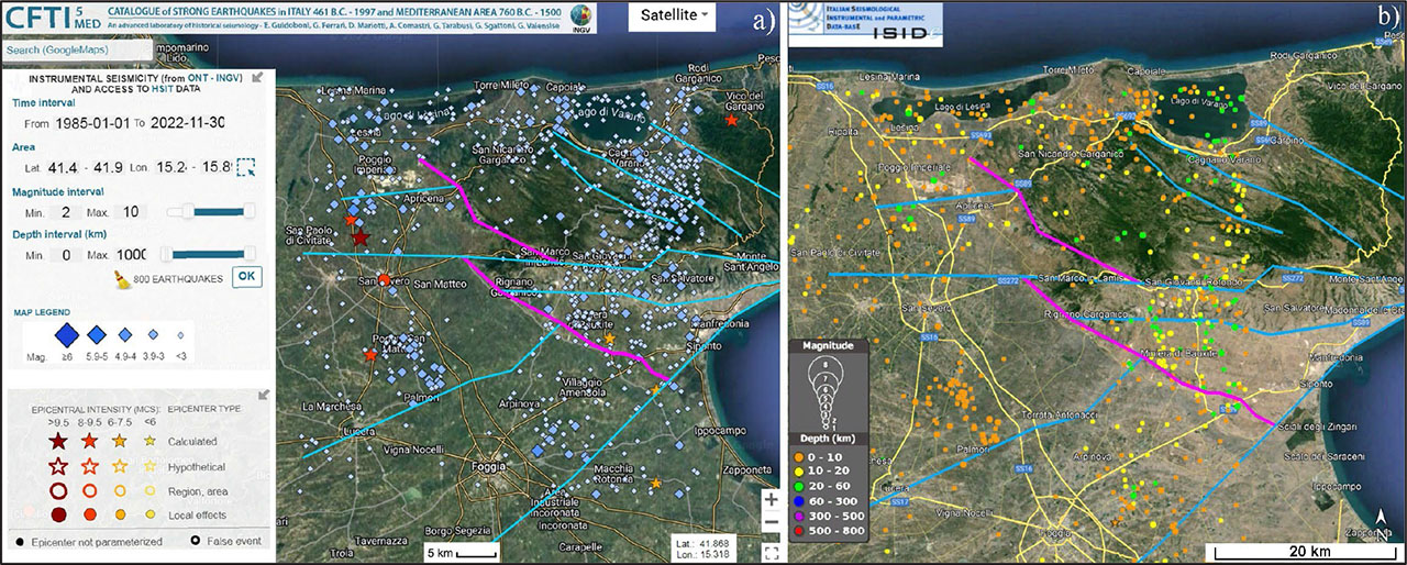
Figure 3:
Seismicity of the ‘Candelaro’ fault area: a) historical and instrumental seismicity (from: [33, 34] modified) and b) depth and magnitude of earthquakes (from: [39] modified).
Table 1:
Input parameters for searching accelerograms in the seismological European Strong-motion database.
| Acceleration component | Magnitude range | Epicentral distance range (km) | Site class | Topographic class | Nominal life (years) | Usage class | Limit state | Scaled records |
|---|---|---|---|---|---|---|---|---|
| Horizontal | 5.6–7 | 0–20 | A | T1 | 50 | II | SLV | No |
| Vertical | 5.2–7 | 0–30 | A | T1 | 50 | II | SLV | Yes |
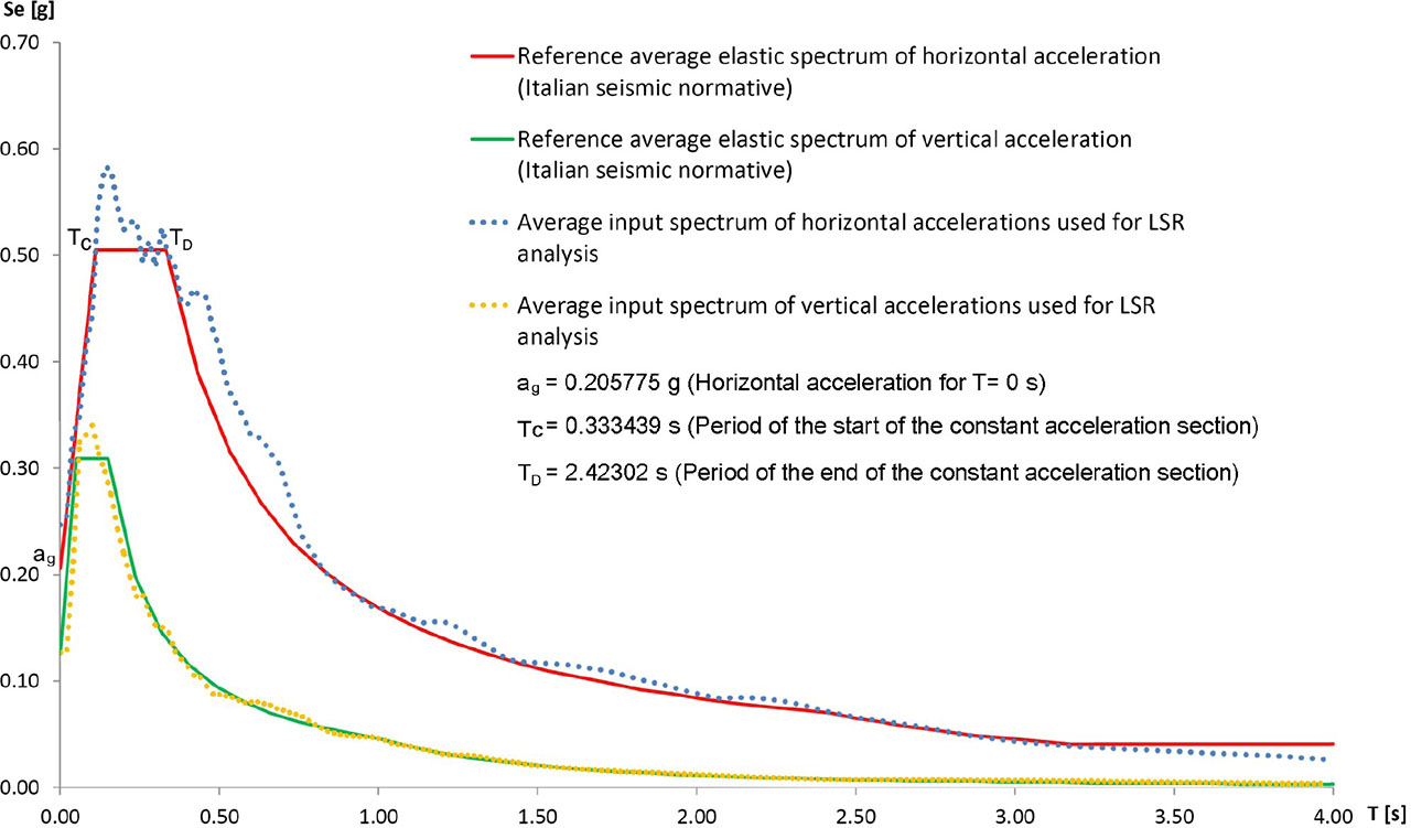
Figure 4:
Average input spectra of horizontal and vertical accelerations used for LSR analysis, compared with elastic spectra for rigid substrate of cat. ‘A’ and horizontal topography [52].
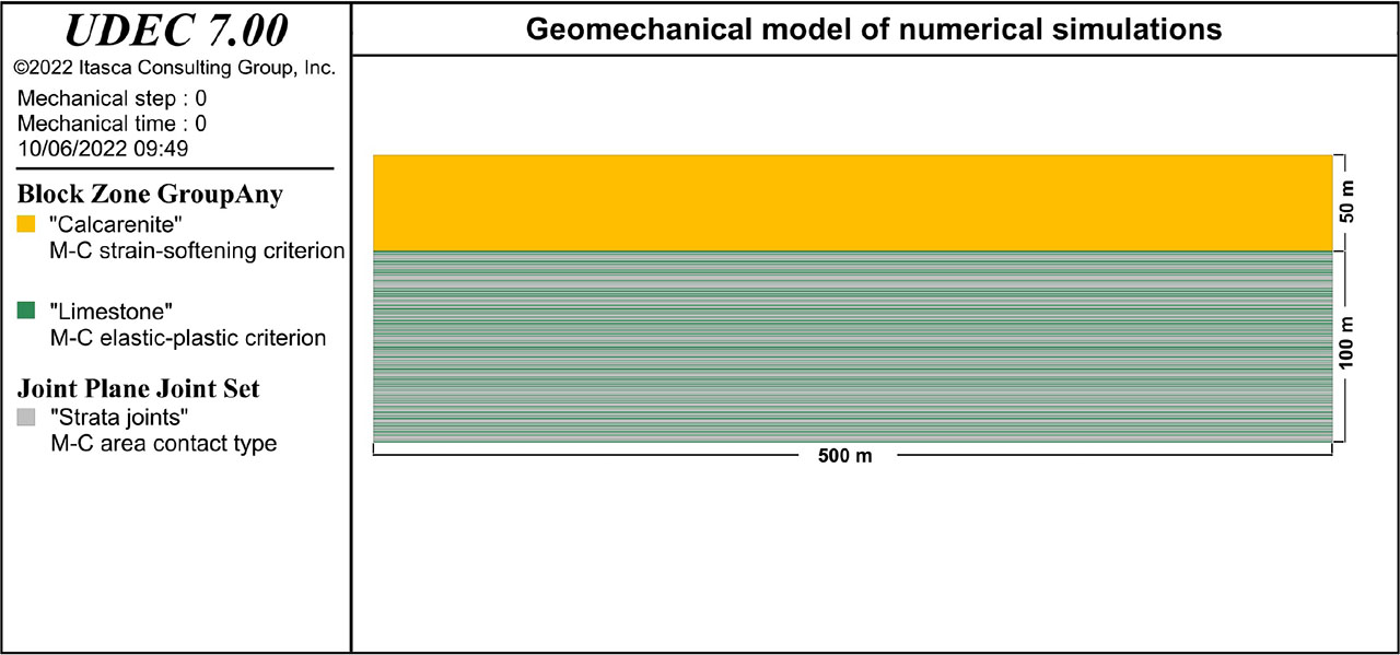
Figure 5:
Geomechanical model used for numerical simulations.
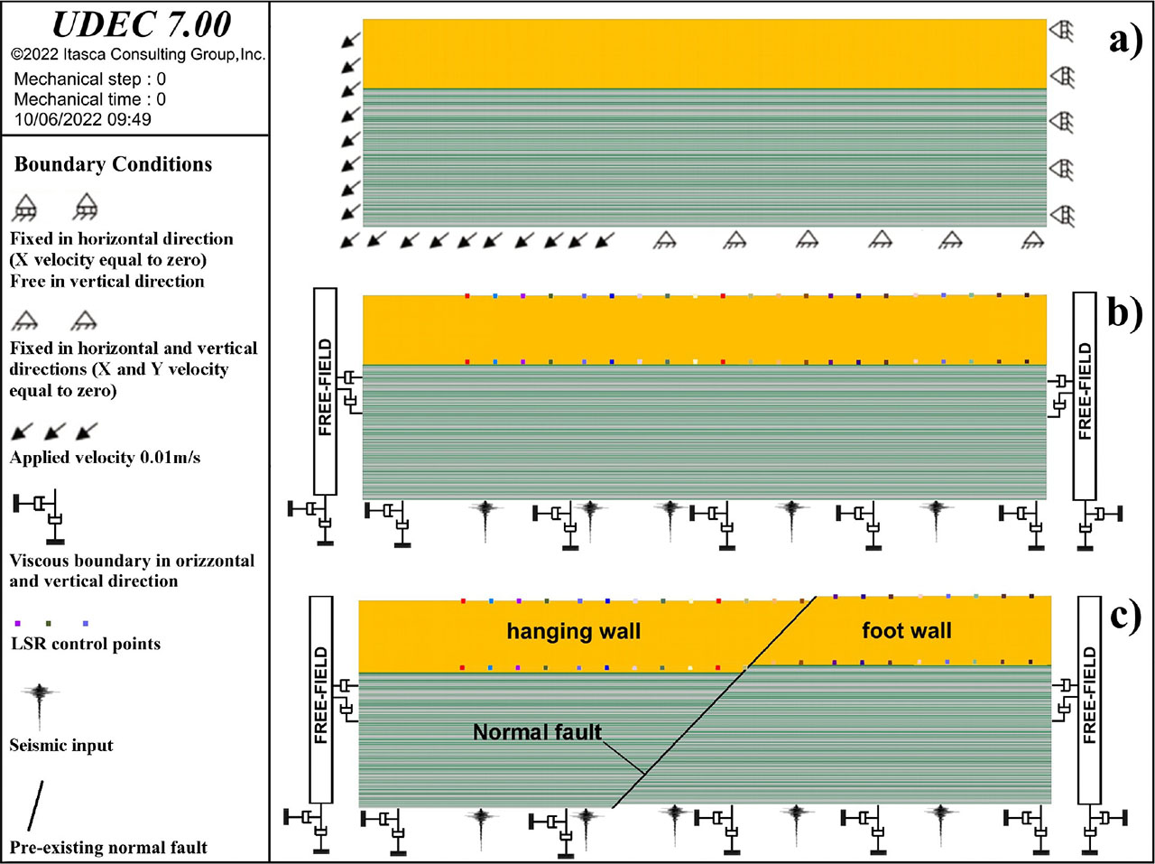
Figure 6:
Models and boundary conditions used in the numerical analyses: a) quasi-static; b) dynamic and LSR (model without pre-existing fault); c) dynamic and LRS (case study with reactivation of a pre-existing normal fault plane 45° dip).
Table 2:
Minimum, maximum and residual values of calcarenite physical–mechanical parameters (from: [5], [15], [17], [23], [26], [59]).
| Physical–mechanical parameters for Mohr–Coulomb Strain-Softening criterion | |||||||||||
|---|---|---|---|---|---|---|---|---|---|---|---|
| Lithotype | Natural unit weight γa (kN/m3) | Porosity nmin - nmax (%) | Imbibition coefficient Cimin - Cimax (%) | Friction angle φres - φmax (degrees) | Cohesion cres - cmax (MPa) | UCS strength σcmax (MPa) | Tensile strength σtres - σtmax (MPa) | Young modulus Emax (GPa) | Bulk modulus Kmax (GPa) | Shear modulus Gmax (GPa) | Dilation angle Δres - Δmax (degrees) |
| Gravina Calcarenite | 19 | 35 – 50 | 15 – 40 | 30 – 38 | 0.13 – 0.29 | 2.0 | 0.11 – 0.26 | 3.5 | 2.9 | 1.3 | 3 – 5 |
Table 3:
Values of physical–mechanical parameters of limestone, layer discontinuities and faults (from: [14], [16], [18]).
| Physical–mechanical parameters for Mohr–Coulomb elasto-plastic criterion | |||||||||
|---|---|---|---|---|---|---|---|---|---|
| Lithotype | Natural unit weight γa (kN/m3) | Friction angle φi (degrees) | Cohesion ci (MPa) | UCS strength σci (MPa) | Tensile strength σti (MPa) | Young modulus Ei (GPa) | Bulk modulus Ki (GPa) | Shear modulus Gi (GPa) | Dilation angle (degrees) |
| Altamura Limestone | 24 | 50 | 13 | 69 | 11 | 60 | 33 | 25 | 7 |
| Mechanical parameters of discontinuities for Mohr–Coulomb ‘area-contact’ criterion | |||||||||
| Rock mass | Joint type | Joint normal stiffness JKN (GPa/m) | Joint shear stiffness JKS (GPa/m) | Joint tensile strength Jtens (MPa) | Joint friction angle Jfric (degrees) | Joint cohesion Jcoh (MPa) | Layers dip (degrees) | Layers spacing (m) | Joint dilation angle (degrees) |
| Altamura Limestone | Layers and faults | 249 | 104 | 0.70 | 39 | 5.29 | 0 | 0.80 | 7 |
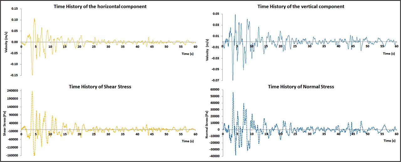
Figure 7:
Time histories of the seismic waves input: horizontal ground motion and shear stress (left); vertical ground motion and normal stress (right).
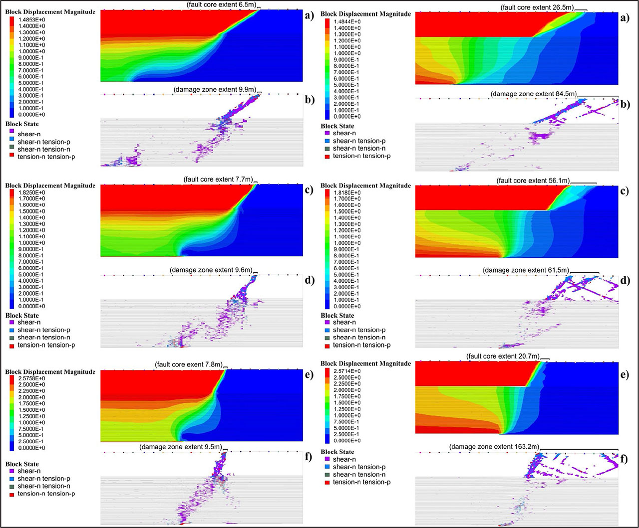
Figure 8:
Displacements, fault core and damage zone extents and plastic states in quasi-static analyses of normal fault generation (left) and reverse fault (right): a–b (dip angle 30°); c–d (dip angle 45°); e–f (dip angle 60°).
Table 4:
Quasi-static analyses: failure types, maximum displacement values, extents of fault core and damage zone.
| Kinematism | Dip angles (degrees) | Type of failure | Maximum displacement on the ground level (m) | Extent of fault core zone on the ground level (m) | Extent of the damage zone on the ground level (m) |
|---|---|---|---|---|---|
| Normal fault | 30 | Conjugate failure surfaces | 1.49 | 6.50 | 9.90 |
| 45 | Single failure surface | 1.83 | 7.70 | 9.60 | |
| 60 | Conjugate failure surfaces | 2.58 | 7.80 | 9.50 | |
| Reverse fault | 30 | Trailing imbricate fan and conjugate surfaces | 1.48 | 26.50 | 84.50 |
| 45 | Trailing imbricate fan and conjugate surfaces | 1.82 | 56.10 | 61.50 | |
| 60 | Conjugate failure surfaces | 2.57 | 20.70 | 163.20 |
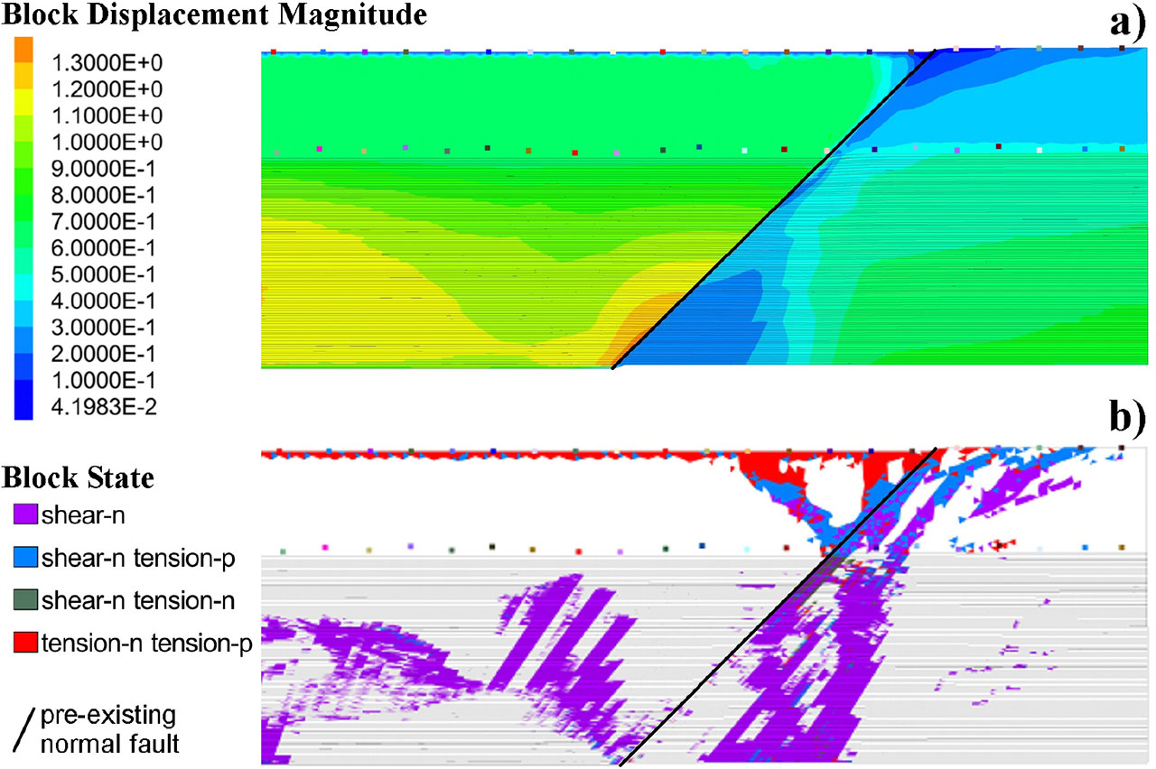
Figure 9:
Dynamic case study analysis of the ‘Candelaro’ active and capable normal fault: a) displacements; b) plastic states.
Table 5:
Dynamic case study analysis of the ‘Candelaro’ active and capable normal fault: failure type, displacement values, extents of fault core and damage zone.
| Kinematism | Dip angles (degrees) | Type of failure | Displacement in depth along the fault plane UDEC simulation (m) | Displacement on the ground level UDEC simulation (m) | Displacement on the ground level equation [2] (m) | Displacement along the fault plane - Hanks and Kanamori’s equation (m) |
|---|---|---|---|---|---|---|
| Normal fault | 45 | Conjugate surfaces ‘Graben o flower structure’ | 0.80–1.30 | 0.1–0.2 | 0.12 | 0.92 |
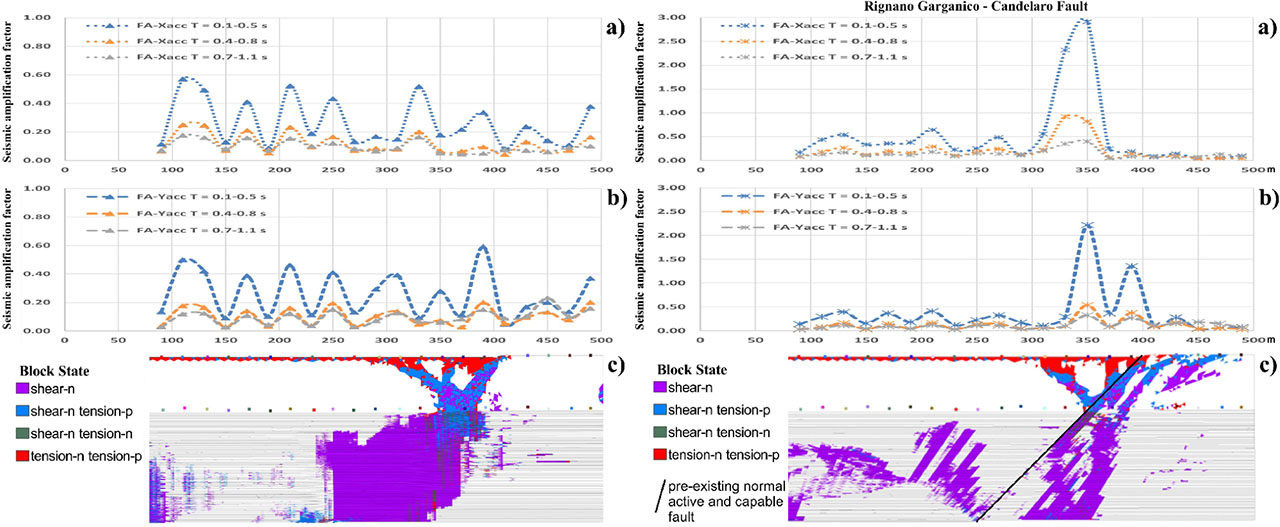
Figure 10:
Local seismic response (LSR) of the case study: on the left model without a pre-existing fault plane – a) FA in X-acceleration, b) FA in Y-acceleration, c) plastic states; on the right model of the ‘Candelaro’ active and capable normal fault plane – a) FA in X-acceleration, b) FA in Y-acceleration, c) plastic states.