
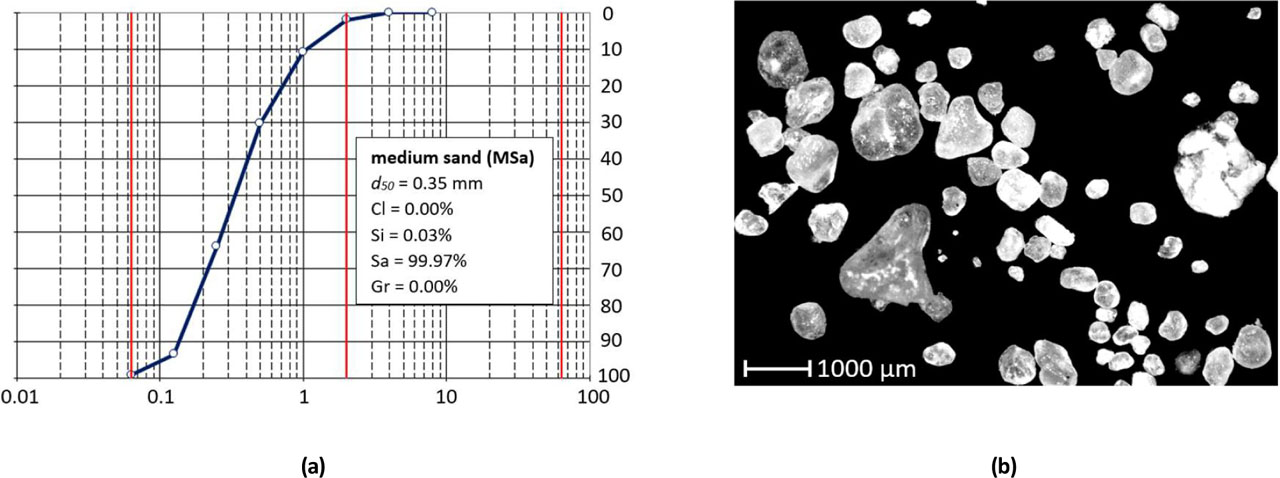
Figure 1:
Tested material (a) grain size distribution (b) microscopic image of tested sand's grains (Dyka, et al., 2017).
Table 1:
The physical parameters of soil.
| Soil type | Gs [-] | d50 [mm] | d60 [mm] | d10 [mm] | CU [-] | emax [-] | emin [-] | ρ [g/cm3] |
|---|---|---|---|---|---|---|---|---|
| silica sand | 2.65 | 0.33 | 0.41 | 0.14 | 3.0 | 0.68 | 0.41 | 1.86 |
[i] Gs—specific gravity (Wichtmann & Triantafyllidis, 2020), dS0, d60, d10—values of the particle diameter at 50, 60, and 10% in the cumulative distribution, CU—uniformity coefficient, emax—maximum void ratio, emin—minimum void ratio, ρ—bulk density
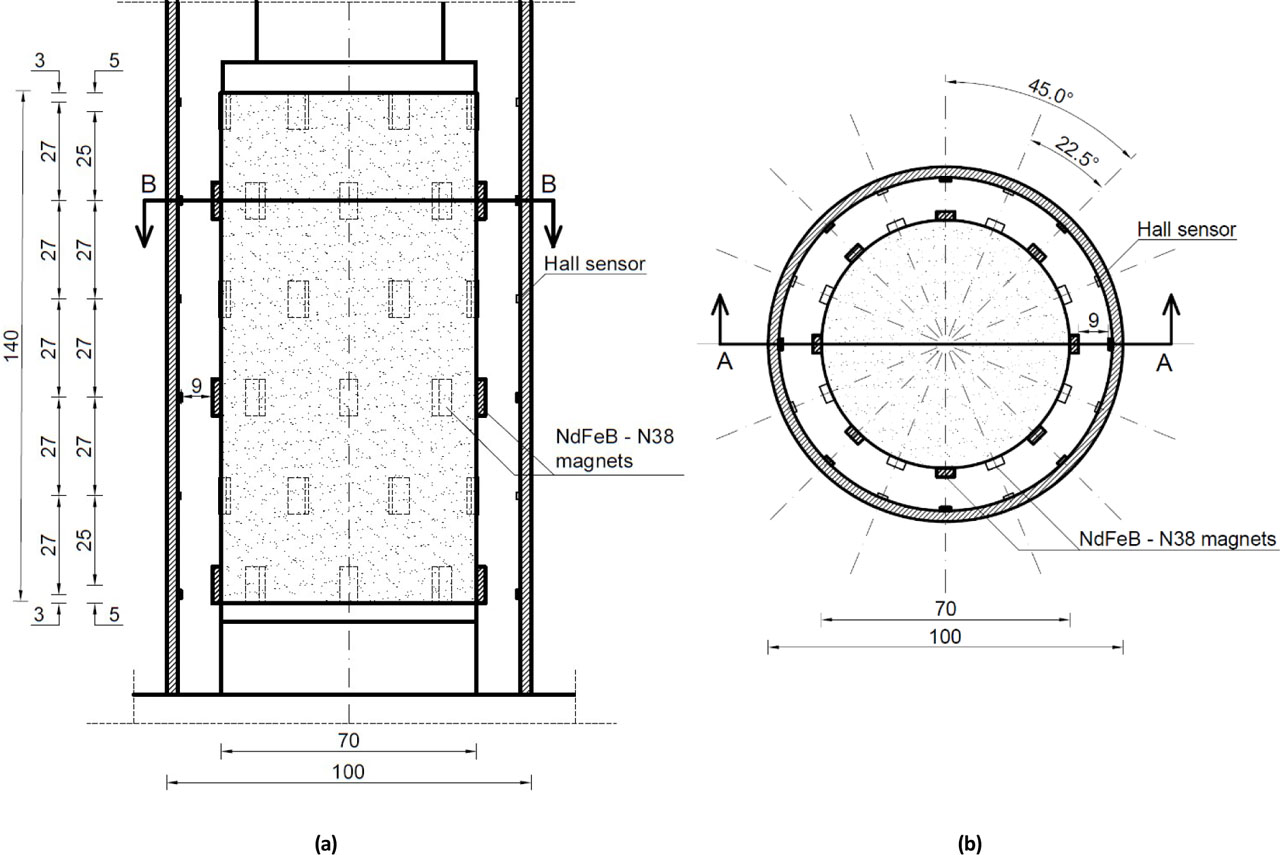
Figure 2:
The arrangement of magnets on the specimen's surface and Hall sensors on the internal cylinder (a) vertical (A-A) section; the middle dimension line refers to the placement of the Hall sensors and the right dimension line refers to the magnets, (b) horizontal (B-B) section [mm].
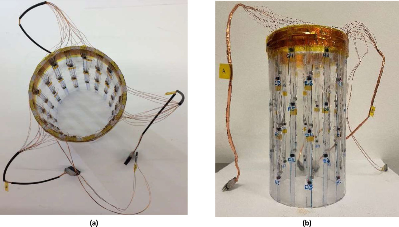
Figure 3:
Polycarbonate cylinder with Hall sensors installed on the surface (a) top view, (b) side view.
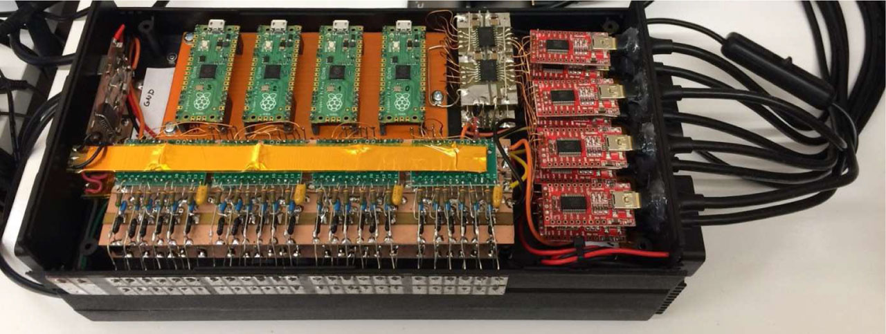
Figure 4:
The inside view of the communications interface.
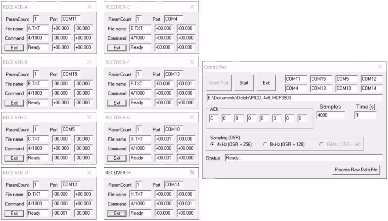
Figure 5:
User Interface of the measurement system control software.
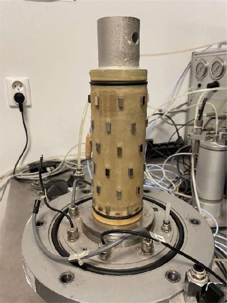
Figure 6:
The sand specimen covered with a latex membrane and magnets attached to the surface The main RC tests were carried out with the input parameters presented in Table 2.
Table 2:
The RC test input parameters.
| Testing mode | Test number | p [kPa] | f0 [Hz] | ff [Hz] | A [V] |
|---|---|---|---|---|---|
| 1. | 100 | 200 | 1.0 | ||
| Resonant column | 2. | 50 | 80 | 180 | 2.0 |
| 3. | 60 | 160 | 3.0 | ||
| 4. | 60 | 160 | 4.0 | ||
| 5. | 50 | 150 | 5.0 | ||
| 6. | 50 | 150 | 6.0 | ||
| 7. | 50 | 150 | 7.0 | ||
| 8. | 40 | 140 | 8.0 |
[i] p—confining pressure, f0—initial frequency (min. value of the frequency spectrum), ff—final frequency (max. value of the frequency spectrum), A—amplitude of torque
Table 3:
The TS test input parameters.
| Testing mode | p [kPa] | f [Hz] | A [V] | n [-] |
|---|---|---|---|---|
| Torsional shearing | 50 | 0.02 | 5.0 | 3 |
[i] p—confining pressure, f—frequency of torque change, A—amplitude of torque, n—number of loading cycles
Table 4:
RC test results.
| RC test number | fr [Hz] | γ [%] | G [MPa] |
|---|---|---|---|
| 1. | 145.45 | 0.0069 | 84.51 |
| 2. | 125.61 | 0.0116 | 62.88 |
| 3. | 115.48 | 0.0144 | 53.27 |
| 4. | 107.60 | 0.0185 | 46.18 |
| 5. | 101.01 | 0.0242 | 40.69 |
| 6. | 96.01 | 0.0312 | 36.73 |
| 7. | 88.81 | 0.0388 | 31.45 |
| 8. | 83.19 | 0.0491 | 27.60 |
[i] fr—resonant frequency, γ—strain, G—shear modulus
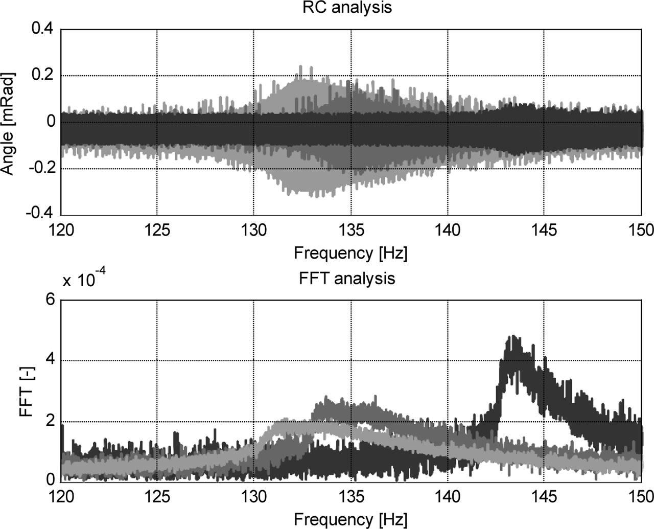
Figure 7:
Influence of the torque amplitude on the resonant frequency of the specimen (light gray—0.02 V, medium gray—0.1 V, black—0.2 V).
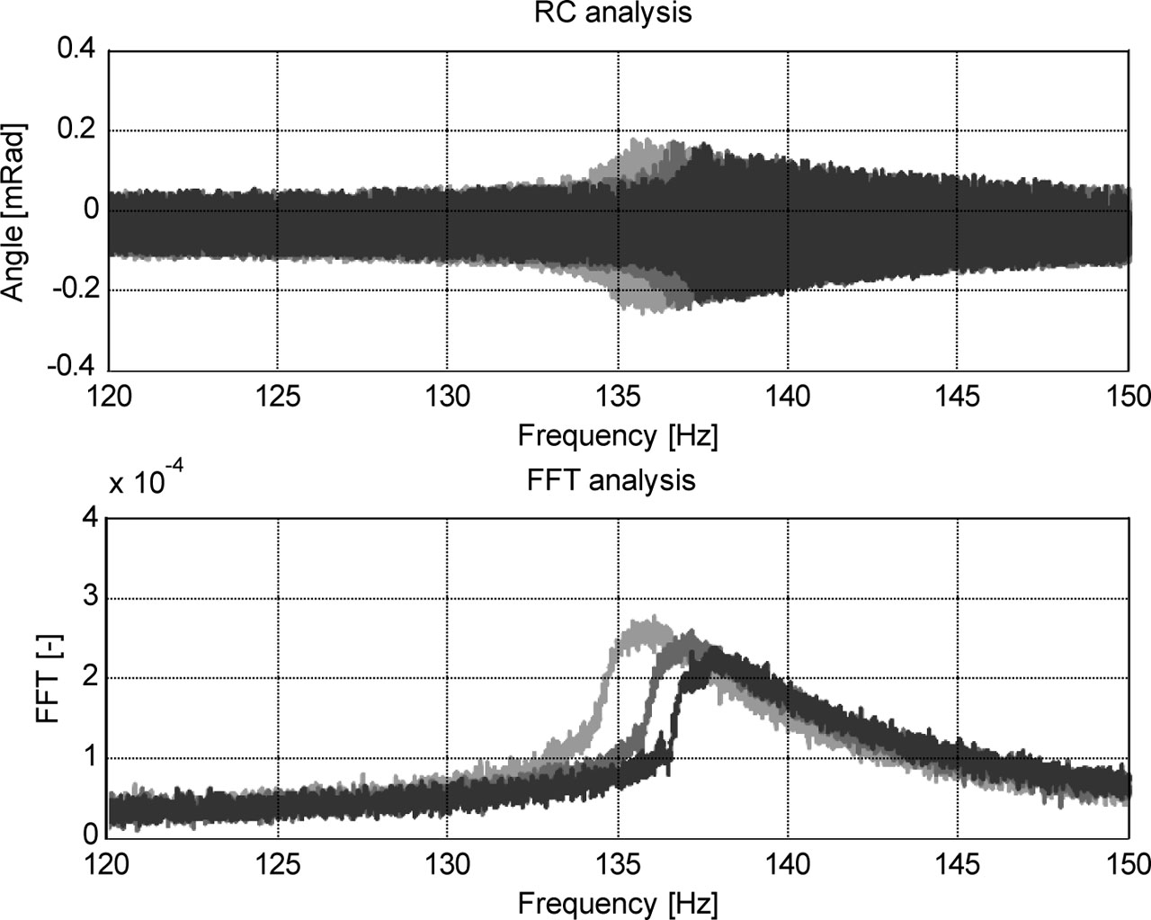
Figure 8:
Influence of the subsequent loading cycles (test repetitions) on the resonant frequency value. The torque amplitude value is 0.2 V; black—first cycle; medium gray—second cycle; light gray—third cycle.
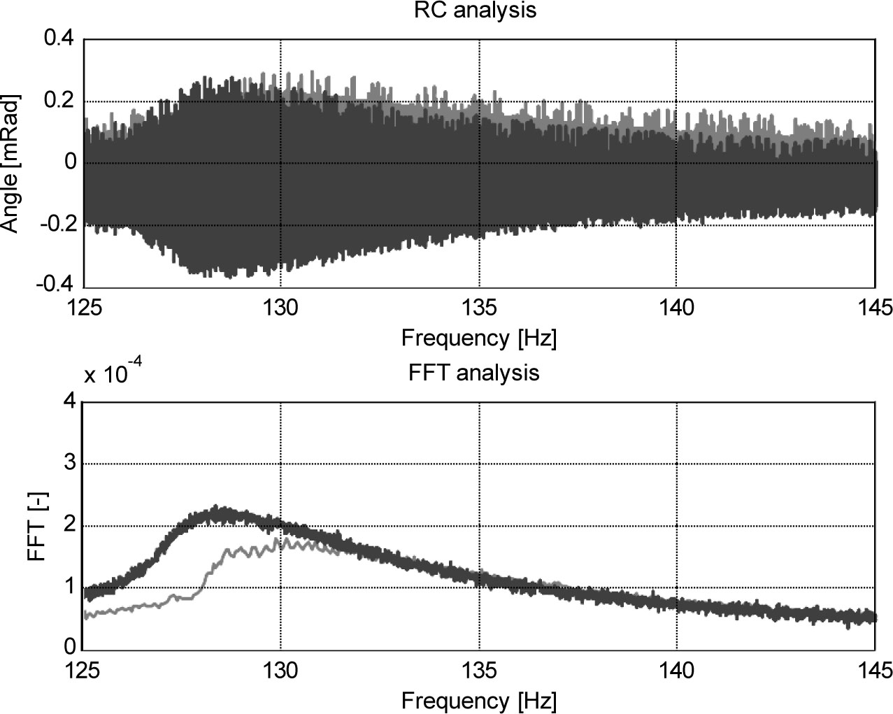
Figure 9:
Influence of the magnets’ installation on the resonant frequency. The torque amplitude is 0.2 V; black—the specimen without magnets; gray—the specimen with the magnets attached to the surface.
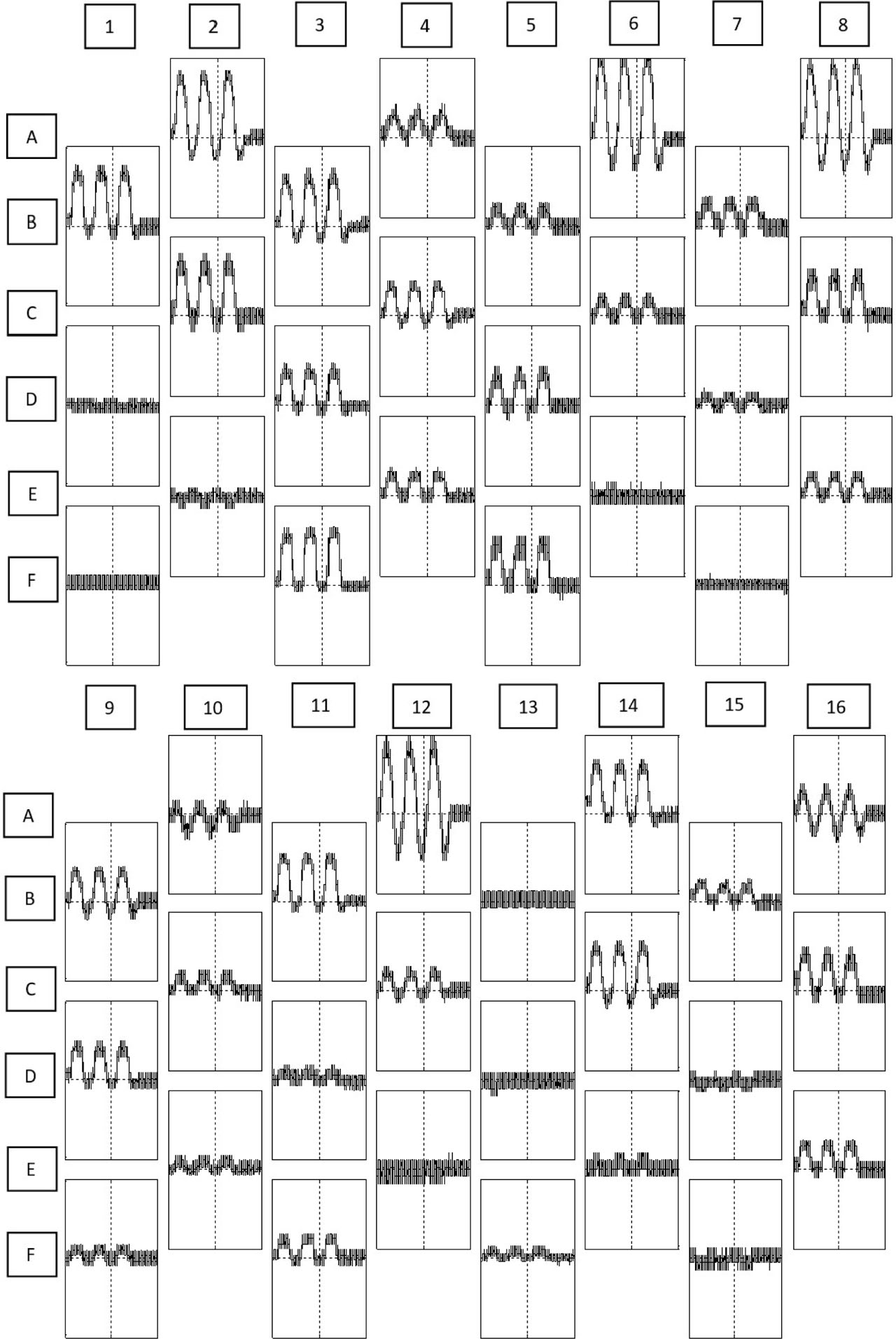
Figure 10:
Results of the TS test for amplitude of 5 V. Raw data from the Hall sensors during the TS test. The arrangement of the graphs corresponds with the location of the sensors.
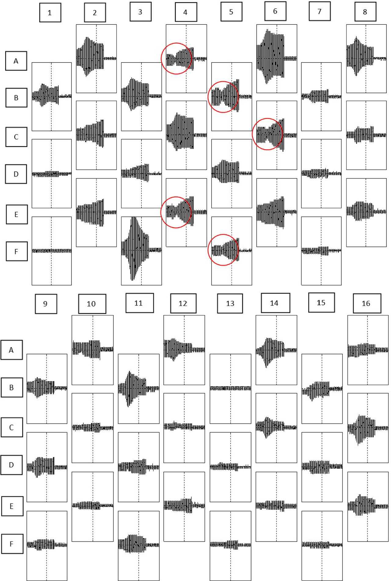
Figure 11:
Results of one of the RC tests for the amplitude of 8 V. Raw data from the Hall sensors. The arrangement of the graphs corresponds with the location of the sensors.