

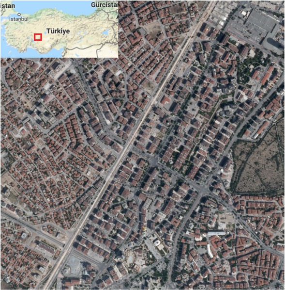
Figure 1
Visualization of the study area
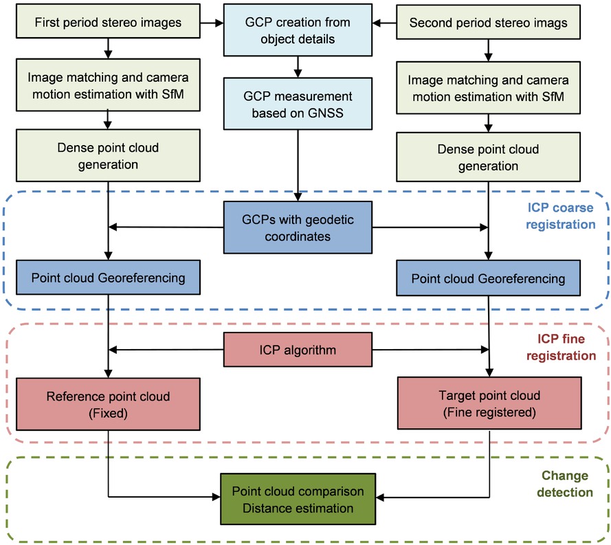
Figure 2
Workflow of the applied change detection method
Table 1
The properties and recording details of the images
| Date | Camera | Focal length [m] | Flying height [m] | Image scale | Image dimensions | Image area [km2] | Stereo area [km2] | Pixel size [micron] |
|---|---|---|---|---|---|---|---|---|
| 1951 | Analogue | 204.18 | 6270 | 30708 | 18 x 18 cm | 46.39 | 27.6 | 23.88 |
| 1975 | Analogue | 208.17 | 7250 | 20000 | 18 x 18 cm | 23.01 | 22.7 | 14.96 |
| 1998 | Analogue | 305 | 5300 | 17377 | 23 x 23 cm | 15.97 | 8.52 | 20.60 |
| 2010 | Digital | 100.50 | 8050 | 80099 | 9420 x 14430 px | 34.26 | 21.7 | 7.20 |
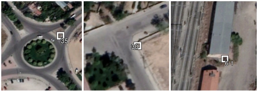
Figure 3
The examples from object-based GCPs
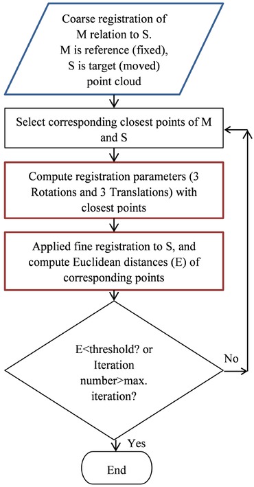
Figure 4
Flowchart of the point cloud registration by the ICP algorithm
Table 2
The informative results of dense point cloud creation
| Year | 1951 | 1975 | 1998 | 2010 |
|---|---|---|---|---|
| Image # | 2 | 3 | 2 | 2 |
| Endlap | 70% | 75% | 70% | 70% |
| Flying altitude [km] | 6.27 | 7.26 | 5.3 | 8.05 |
| Ground res. [cm/px] | 73.4 | 40.3 | 36.6 | 50.2 |
| Coverage area [km2] | 27.6 | 22.7 | 8.52 | 21.7 |
| Tie points | 1616 of | 6527 of | 3817 of | 3870 of |
| 1756 | 6655 | 3988 | 3994 | |
| Projections | 3232 | 13487 | 7634 | 7740 |
| Reproj. err. [px] | 0.989 | 0.867 | 0.686 | 0.259 |
| Max. reproj. err. [px] | 5.804 | 8.034 | 6.59486 | 1.910 |
| Dense points # | 2539040 | 8859870 | 3995753 | 5243623 |
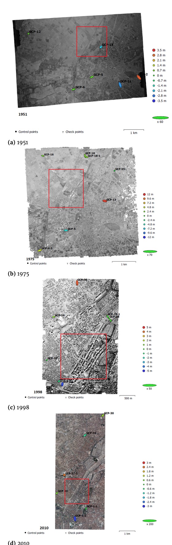
Figure 5
The GCP locations and error estimates on point clouds of a) 1951, b) 1975, c) 1998 and d) 2010. The Z error is represented by ellipse colour. The X, Y errors are represented by ellipses. The estimated GCP locations are shown with a dot or cross. (Red rectangle indicates the study area)
Table 3
The RMSE of residuals on GCP coordinates after the geo-registration [m]
| Date | GCP # | RMSEX | RMSEY | RMSEZ | RMSEXY | RMSEXYZ |
|---|---|---|---|---|---|---|
| 1951 | 6 | 1.54 | 1.60 | 1.86 | 2.22 | 2.90 |
| 1975 | 7 | 1.09 | 1.03 | 3.67 | 1.50 | 3.96 |
| 1998 | 7 | 0.80 | 1.30 | 2.52 | 1.53 | 2.94 |
| 2010 | 6 | 0.32 | 0.52 | 1.62 | 0.61 | 1.73 |
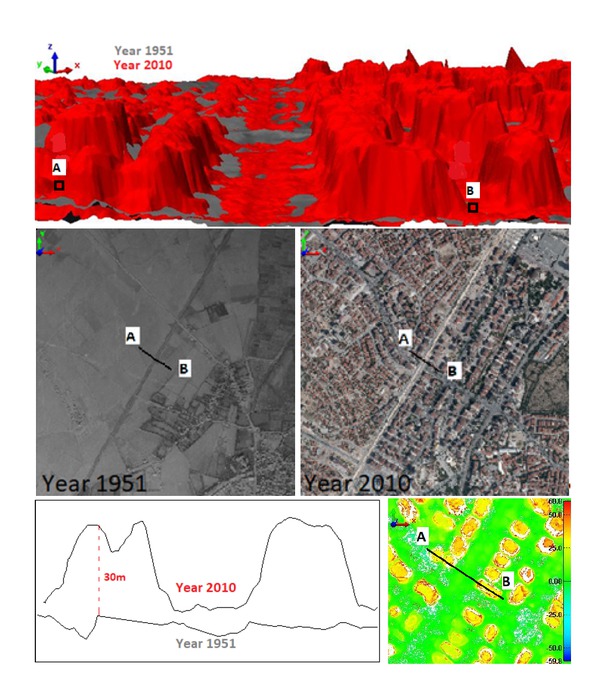
Figure 6
The cross-section from compared data of 1951 and 2010. The height differences correspond to the changes.
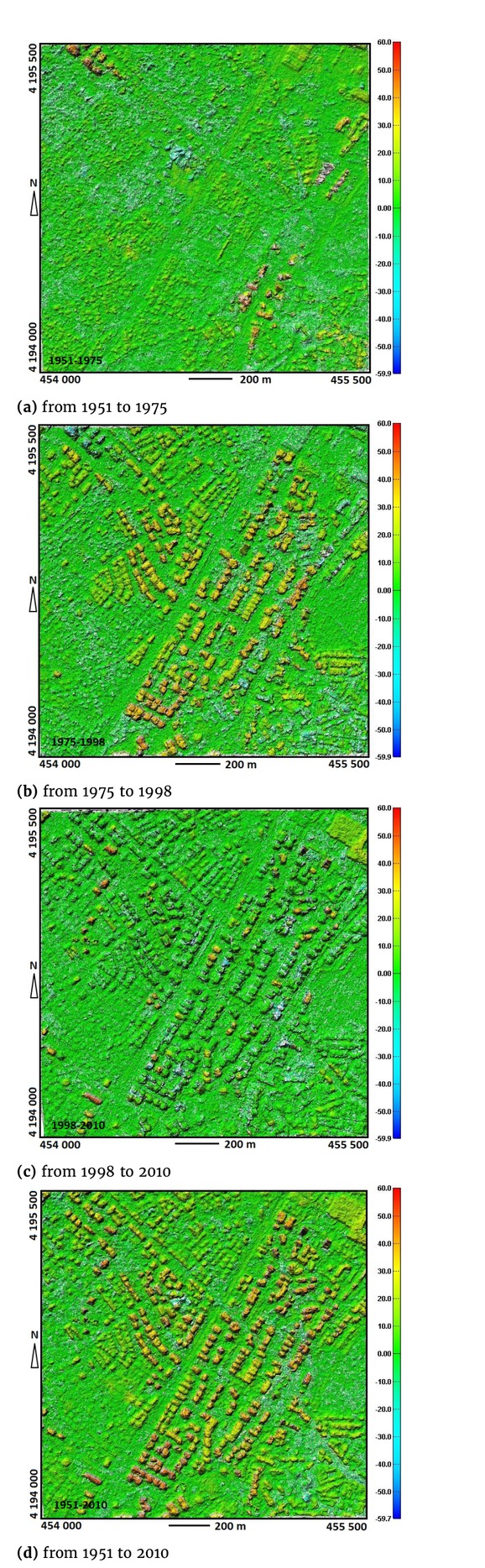
Figure 7
The estimated changes (legend units: meters)
Table 4
The ICP convergence of compared point clouds
| Date comparison | Convolution [m] | Mean [cm] | Std. Dev. [m] |
|---|---|---|---|
| 1951–1975 | 9.2e-7 | 0.06 | 0.99 |
| 1975–1998 | 7.1e-7 | -0.87 | 0.96 |
| 1998–2010 | 9.3e-7 | 0.09 | 0.94 |
| 1951–2010 | 9.1e-7 | 0.12 | 0.99 |
Table 5
The change quantities for the historical periods
| Year | RMSE [m] | Average d [m] | Std. dev. ᓂ [m] |
|---|---|---|---|
| 1951–1975 | 8.42 | 4.82 | 6.91 |
| 1975–1998 | 8.51 | -0.90 | 8.46 |
| 1998–2010 | 9.10 | 6.69 | 6.18 |
| 1951–2010 | 14.16 | 10.60 | 9.39 |
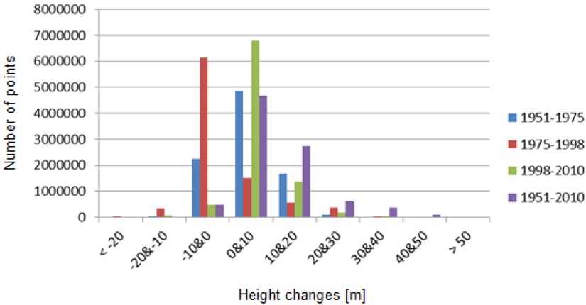
Figure 8
The change comparison during the historical periods
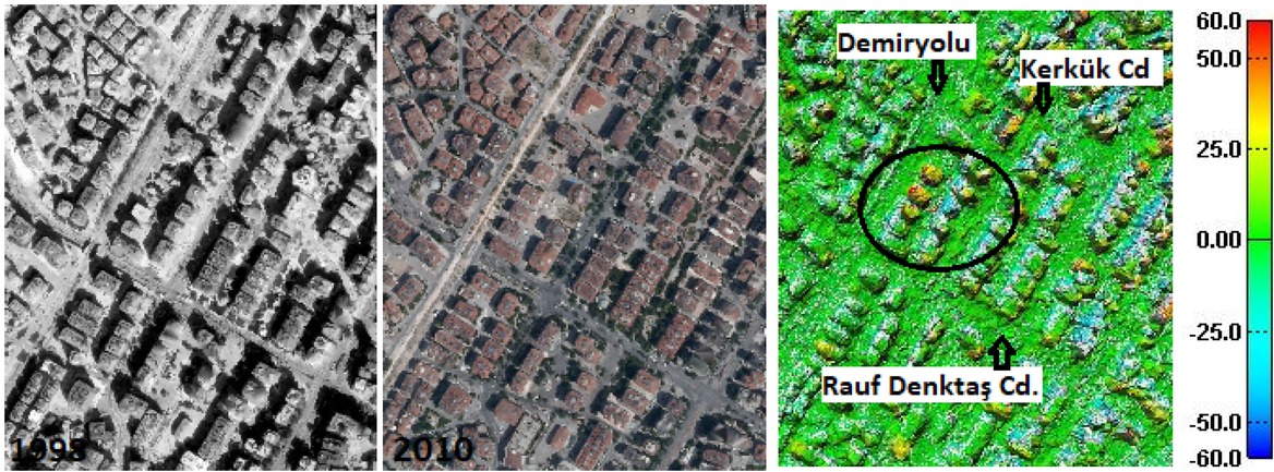
Figure 9
The changes due to demolished and new buildings from 1998 to 2010 (Unit: meter)
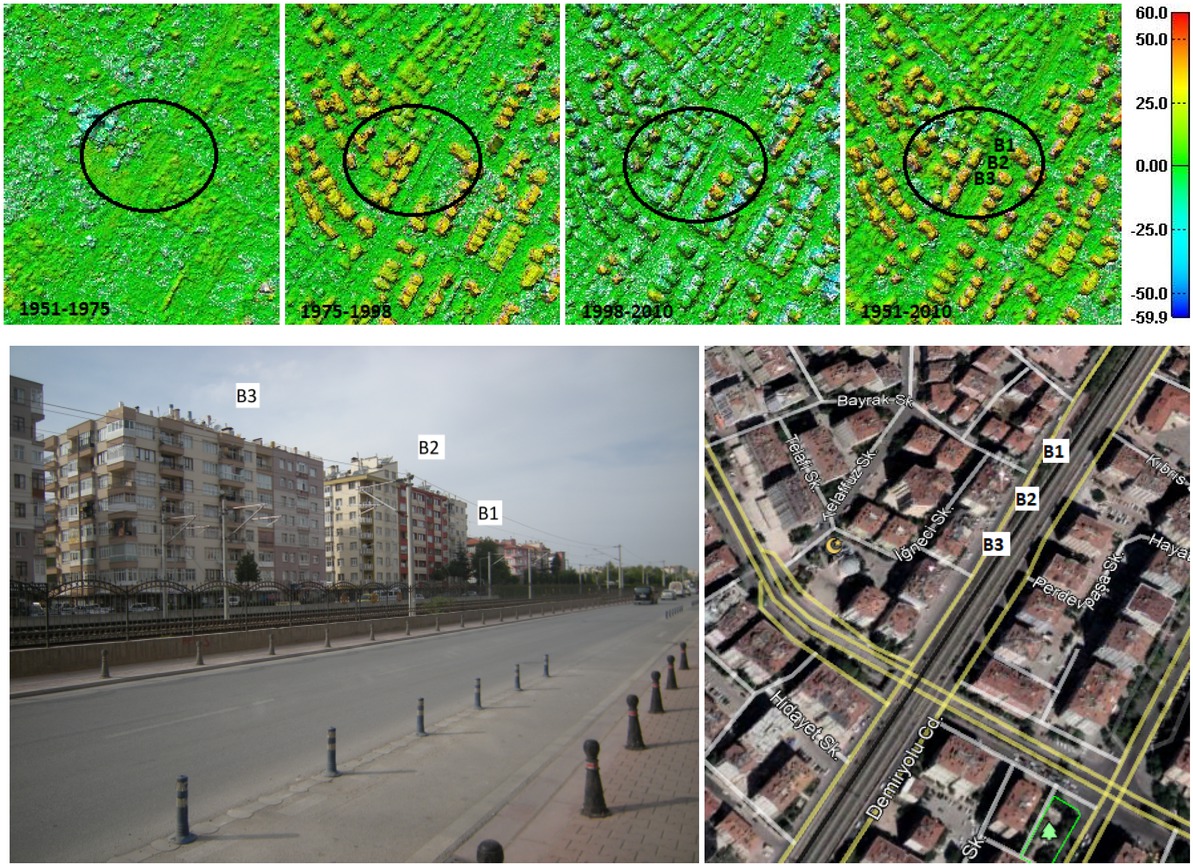
Figure 10
The visualization of changes in comparison of time series point clouds (B1 location: 37°53’09.15”N latitude, 32°29’08.37”E longitude) (Legend unit: meter)