

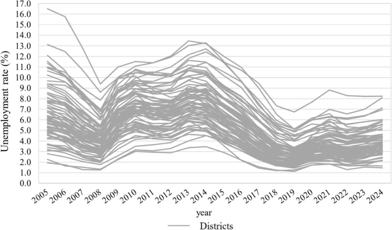
Fig. 1:
The development of unemployment rate across Czech districts (2005–2024, annual averages); author’s elaboration using data from MoLSA (2025)
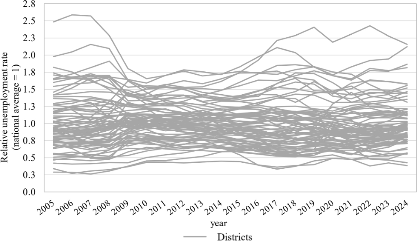
Fig. 2:
The development of relative unemployment rate across Czech districts (2005–2024, annual averages, national average = 1); author’s elaboration using data from MoLSA (2025)
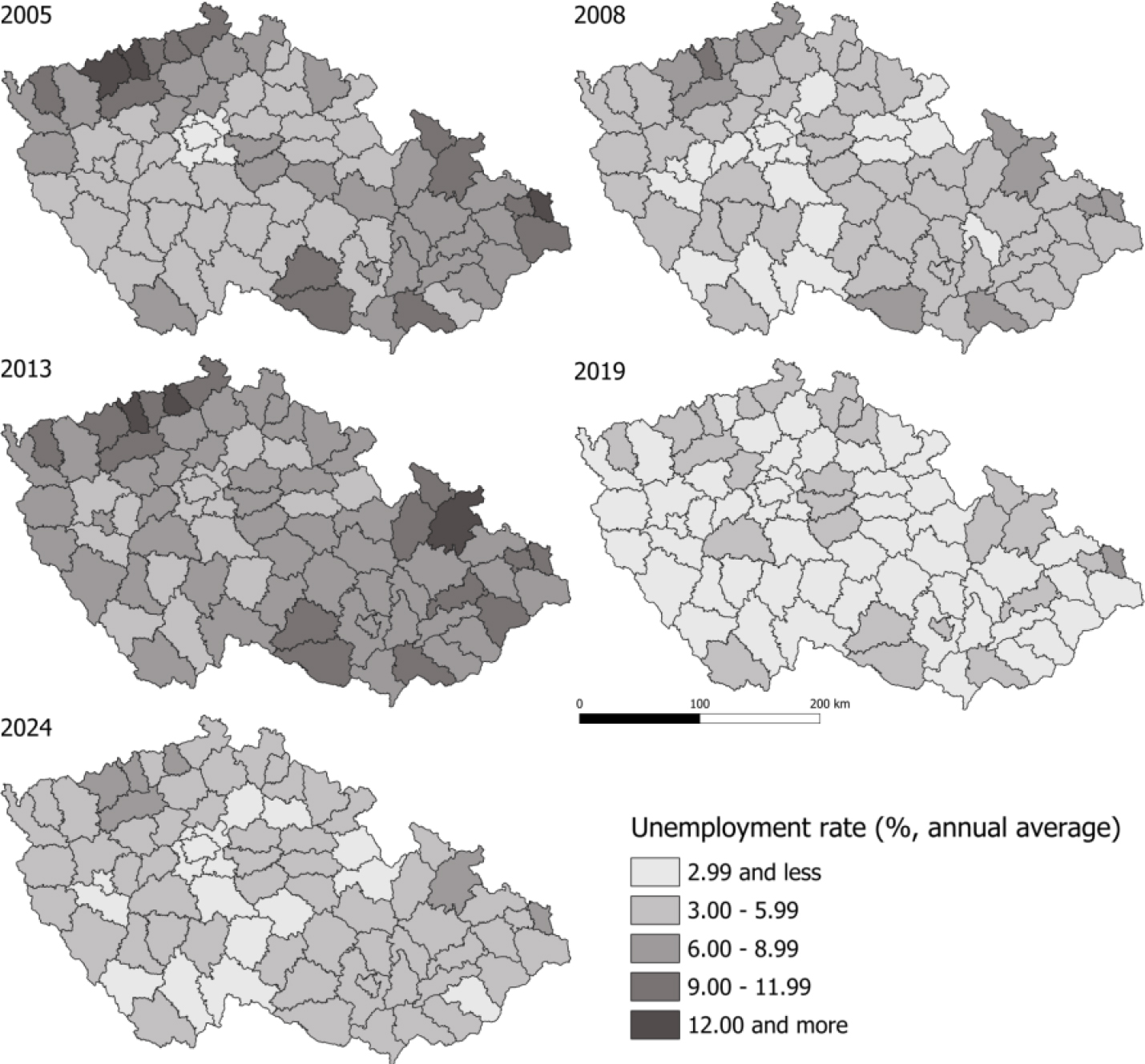
Fig. 3:
Development of unemployment rates across Czech districts in selected years (annual averages, %);author’s elaboration using data from MoLSA (2025) using shapefile from ČÚZK (2022), own elaboration in QGIS 3.36.0-Maidenhead (QGIS.org, 2024), Mapový podklad – Soubor hranic, 2022 © Český úřad zeměměřický a katastrální, www.cuzk.cz (ČÚZK, 2022)
Tab. 1:
Absolute β-convergence model for district-level unemployment, OLS estimates (p-values reported in parentheses)
| 2005–2008 | 2008–2013 | 2013–2019 | 2019–2024 | 2005–2024 | |
|---|---|---|---|---|---|
| α (constant) | – 0.1242 (0.000) | 0.2323 (0.000) | –0.2384 (0.000) | 0.0966 (0.000) | 0.0007 (0.891) |
| β (initial unemployment) | –0.0158 (0.201) | –0.0732 (0.000) | 0.0294 (0.022) | –0.0296 (0.000) | –0.0156 (0.000) |
| F test | 1.67 (0.2005) | 206.60 (0.0000) | 5.46 (0.0221) | 16.11 (0.0001) | 35.37 (0.0000) |
| R2 | 0.0218 | 0.7337 | 0.0679 | 0.1768 | 0.3205 |
| White’s test (heteroskedasticity) | 1.75 (0.4169) | 1.25 (0.5359) | 0.04 (0.9783) | 5.00 (0.0820) | 0.26 (0.8787) |
| Breusch-Pagan/Cook-Weisberg test (heteroskedasticity) | 0.07 (0.7978) | 1.37 (0.2410) | 0.00 (0.9886) | 4.53 (0.0333) | 0.18 (0.6693) |
| Skewness/Kurtosis tests for normality (residuals) | 8.03 (0.0180) | 0.85 (0.6526) | 0.30 (0.8601) | 1.37 (0.5029) | 1.53 (0.4655) |
1 Source: Author’s calculations in Stata 15 (StataCorp, 2017)
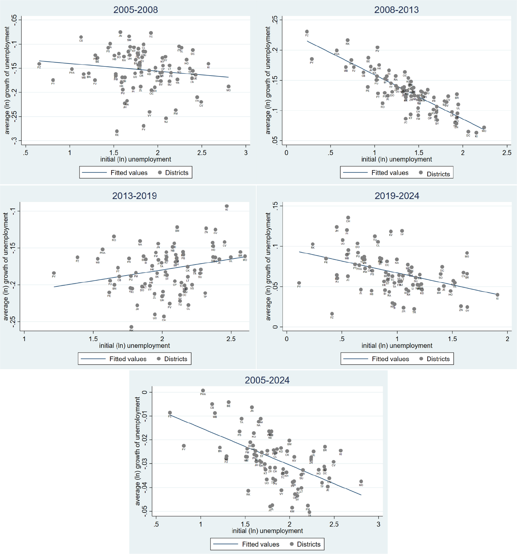
Fig. 4:
Graphical depiction of absolute β-convergence of unemployment rates across Czech districts, 2005–2024; author’s processing in Stata 15 (StataCorp, 2017) based on data from MoLSA (2025)
Tab. 2:
Spatial lag β-convergence model for district-level unemployment, Maximum Likelihood estimates (p-values reported in parentheses)
| 2005–2008 | 2008–2013 | 2013–2019 | 2019–2024 | 2005–2024 | |
|---|---|---|---|---|---|
| α (constant) | –0.0766 (0.004) | 0.2335 (0.000) | –0.1874 (0.000) | 0.0759 (0.000) | 0.0030 (0.537) |
| β (initial unemployment) | –0.0076 (0.516) | –0.0734 (0.000) | 0.0297 (0.013) | –0.0304 (0.000) | –0.0125 (0.000) |
| ρ (spatial autoregressive parameter) | 0.4089 (0.003) | –0.0065 (0.952) | 0.2870 (0.060) | 0.3178 (0.020) | 0.2875 (0.028) |
| Direct effect | –0.0079 (0.514) | –0.0734 (0.000) | 0.0303 (0.014) | –0.0311 (0.000) | –0.0127 (0.000) |
| Indirect effect | –0.0049 (0.507) | 0.0005 (0.952) | 0.0114 (0.231) | –0.0134 (0.134) | –0.0048 (0.067) |
| Total effect | –0.0128 (0.505) | –0.0729 (0.000) | 0.0417 (0.030) | –0.0446 (0.001) | –0.0175 (0.000) |
| Wald χ2 test | 10.55 (0.0051) | 212.13 (0.0000) | 9.51 (0.0086) | 23.40 (0.0000) | 43.98 (0.0000) |
| Pseudo R2 | 0.0375 | 0.7337 | 0.0494 | 0.1418 | 0.3491 |
| Moran test for spatial dependence | 7.16 (0.0074) | 0.02 (0.8933) | 5.54 (0.0186) | 10.48 (0.0012) | 1.88 (0.1698) |
1 Source: Author’s calculations in Stata 15 (StataCorp, 2017)
Tab. 3:
Summary of results
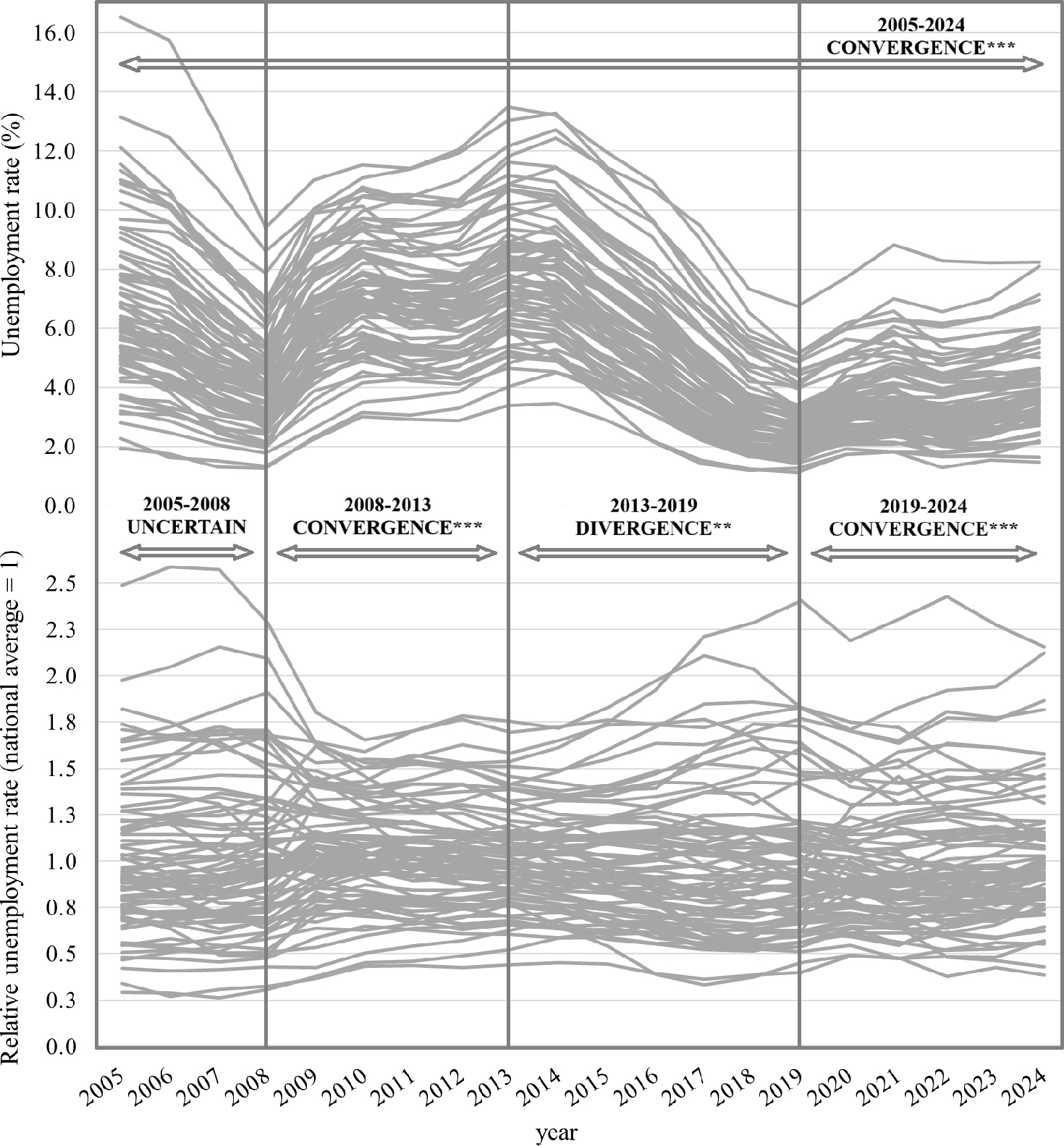
Fig. 5:
Graphical depiction of results – unemployment dynamics across Czech districts, 2005–2024; author’s elaboration based on results of econometric analysis and using data from MoLSA (2025)
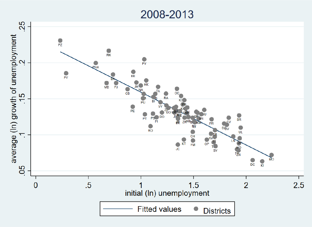
Fig. 6:
Graphical depiction of absolute β-convergence of unemployment rates across Czech districts, 2008–2013; author’s processing in Stata 15 (StataCorp, 2017) based on data from MoLSA (2025)
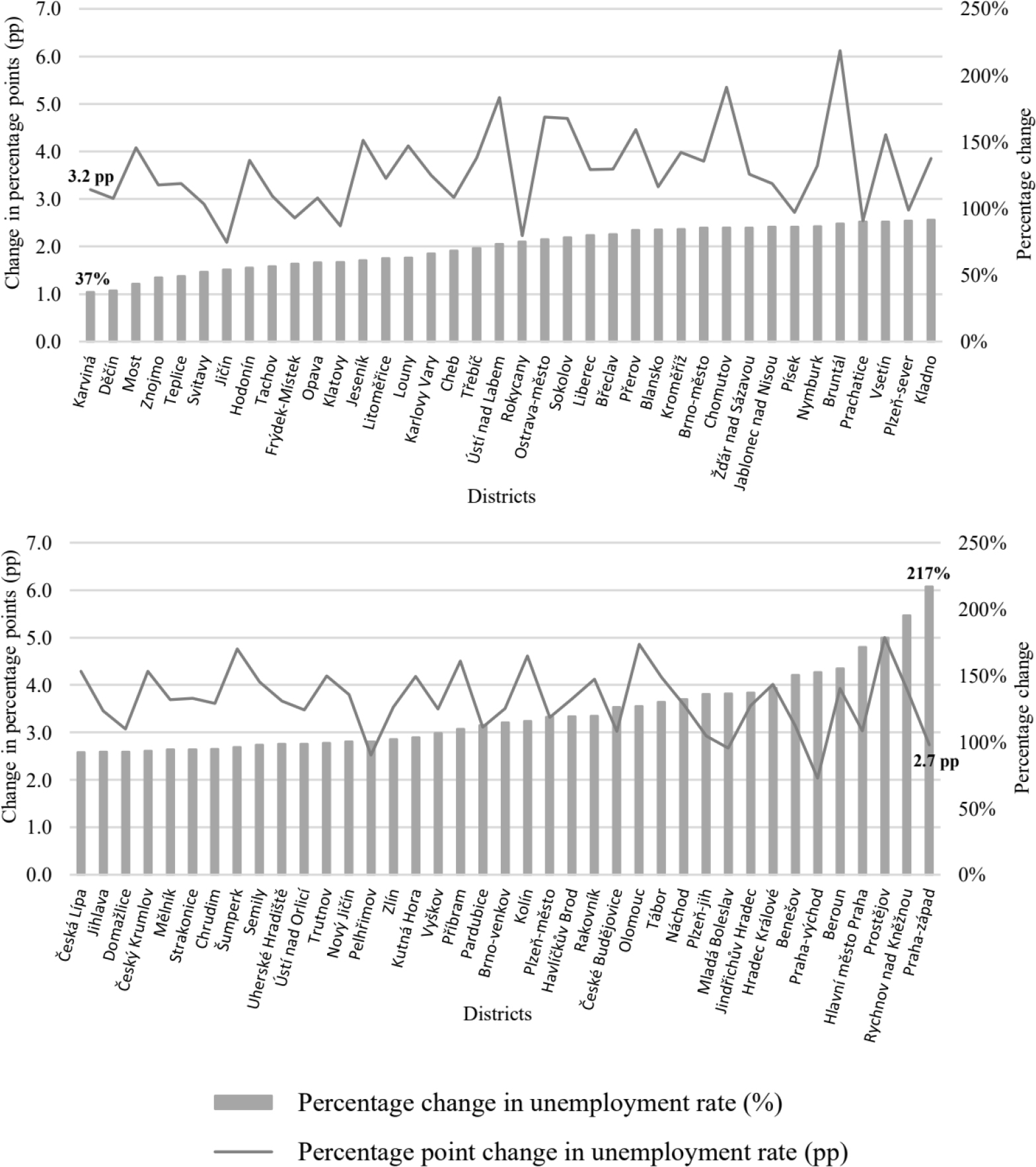
Fig. 7:
Change of unemployment rate across Czech districts (2008–2013), comparison of absolute change (percentage points, pp) and relative change (%); author’s elaboration using data from MoLSA (2025)