
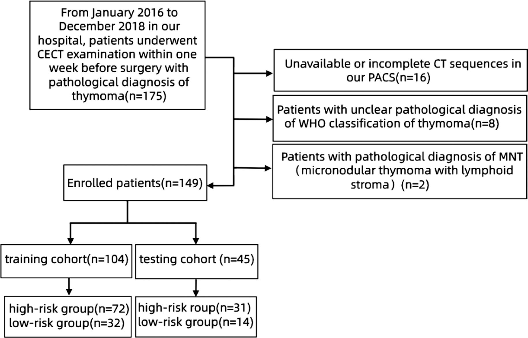
FIGURE 1.
The flow chart of the case selection process
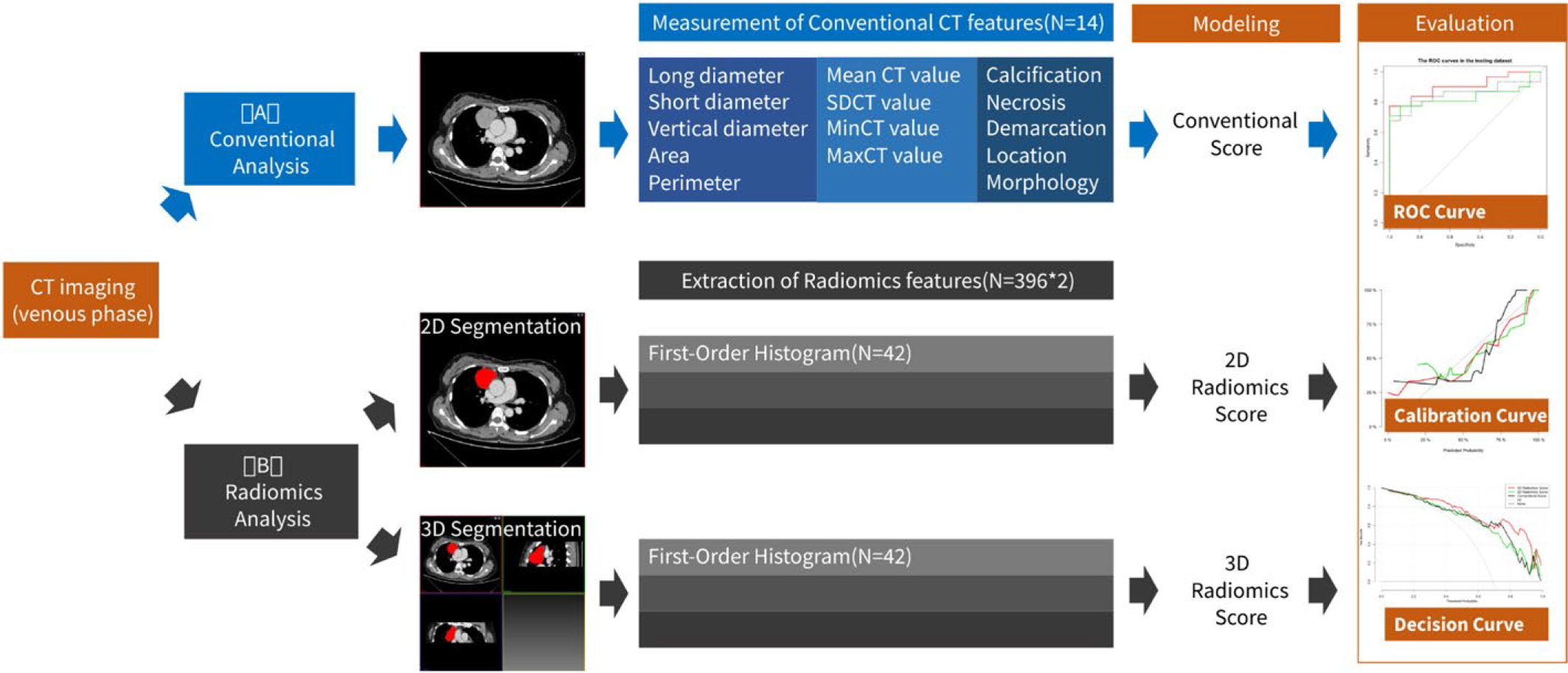
Figure 2.
The flow chart of the CT imaging analysis. (A) shows the workflow of conventional analysis and 14 conventional features were recorded. (B) shows the workflow of radiomics analysis. 2D and 3D segmentation were performed on the CT images and 396 radiomics features were extracted respectively. The most predictive feature variables were selected, and the multivariate logistic regression analysis was applied to build the prediction models. The predicting abilities of the conventional and radiomics models were demonstrated by receiver operating characteristic (ROC) curves. The goodness of fit was assessed using calibration curve of the Hosmer-Lemeshow test. Additionally, decision curve analysis (DCA) was conducted to determine the clinical usefulness of the models.
Table 1.
Baseline characteristics of the patients in training and testing dataset
| Training set | Testing set | |||||
|---|---|---|---|---|---|---|
| Low-risk (n=32) | High-risk (n= 72) | P | Low-risk (n=14) | High-risk (n=31) | P | |
| Age, (Mean ± SD) years | 53.6±11.2 | 52.5±11.4 | 0.656 | 54.0±10.7 | 56.4±8.9 | 0.446 |
| Sex (male, No. (%)) | 14 (43.8) | 37 (51.4) | 0.472 | 7 (50.0) | 18 (58.1) | 0.614 |
| Myasthenia gravis, No. (%) | 7 (21.9) | 24 (33.3) | 0.238 | 0 (0.0) | 8 (25.8) | 0.094 |
| Thoracalgia, No. (%) | 3 (9.4) | 18 (25.0) | 0.067 | 1 (7.1) | 11 (35.5) | 0.104 |
Table 2.
Distribution of conventional CT features in training and testing dataset
| Testing set | Training set | |||||
|---|---|---|---|---|---|---|
| Low-risk (n=32) | High-risk (n= 72) | P | Low-risk (n=14) | High-risk (n=31) | P | |
| Mean CT value (HU) | 79.5 (68.4, 91.6) | 62.0 (51.0, 78.8) | <0.001 | 88.5 (76.0, 95.1) | 67.0 (59.2, 74.0) | <0.001 |
| Standard deviation | 18.0 (16.0, 22.6) | 16.5 (14.0, 19.0) | 0.050 | 18.0 (15.9, 26.2) | 17.0 (14.2, 21.6) | 0.548 |
| Minimum CT value (HU) | -6.10±30.2 | -8.5±25.0 | 0.678 | -0.7±31.6 | -7.3±17.9 | 0.477 |
| Maximum CT value (HU) | 148.5 (131.0, 172.1) | 118.0 (105.5, 138.6) | <0.001 | 162.0 (148.9, 166.1) | 129.0 (105.4, 146.8) | 0.002 |
| Long diameter (mm) | 50.6±17.0 | 44.1±19.4 | 0.106 | 47.8 (40.9, 57.8) | 38.0 (27.7, 61.3) | 0.198 |
| Short diameter (mm) | 34.7 (23.9, 41.7) | 23.2 (17.7, 34.6) | 0.009 | 36.5 (26.0, 45.4) | 25.6 (19.0, 39.3) | 0.073 |
| Vertical diameter (mm) | 48.6 (44.1, 60.2) | 40.4 (29.1, 55.2) | 0.204 | 50.5 (44.4, 63.6) | 38.9 (33.1, 55.1) | 0.059 |
| Area (mm2) | 1321.5 (692.0, 1889.8) | 628.5 (397.4, 1409.7) | 0.008 | 1024.0 (747.7, 1623.3) | 651.0 (346.0, 1362.8) | 0.315 |
| Perimeter (mm) | 143.0 (110.8, 167.7) | 112.5 (78.6, 153.8) | 0.021 | 143.5 (118.6, 255.4) | 100.0 (84.1, 194.8) | 0.098 |
| Location | 0.373 | 0.790 | ||||
| Right mediastinum | 10 (31.3%) | 33 (45.8%) | 7 (50.0%) | 11 (35.5%) | ||
| Middle | 8 (25.0%) | 15 (20.8%) | 1 (7.1%) | 3 (9.7%) | ||
| Left mediastinum | 14 (43.8%) | 24 (33.3%) | 6 (42.9%) | 17 (54.8%) | ||
| Morphology | 0.010 | <0.001 | ||||
| Lobular | 5 (15.6%) | 10 (13.9%) | 7 (50.0%) | 2 (6.5%) | ||
| Shallowly-lobulated | 15 (46.9%) | 14 (19.4%) | 7 (50.0%) | 15 (48.4%) | ||
| Non-lobular | 12 (37.5%) | 48 (66.7%) | 0 (0.0%) | 14 (45.2%) | ||
| Demarcation | 0.023 | 0.010 | ||||
| Clear | 15 (46.9%) | 17 (23.6%) | 10 (71.4%) | 8 (25.8%) | ||
| Unclear | 16 (50.0%) | 43 (59.7%) | 4 (28.6%) | 17 (54.8%) | ||
| Infiltration | 1 (3.1%) | 12 (16.7%) | 0 (0%) | 6 (19.4%) | ||
| Internal calcification | 8 (25.0%) | 13 (18.1%) | 0.416 | 4 (28.6%) | 9 (29.0%) | 0.746 |
| Necrosis | 12 (37.5%) | 20 (27.8%) | 0.321 | 9 (64.3%) | 12 (38.7%) | 0.111 |
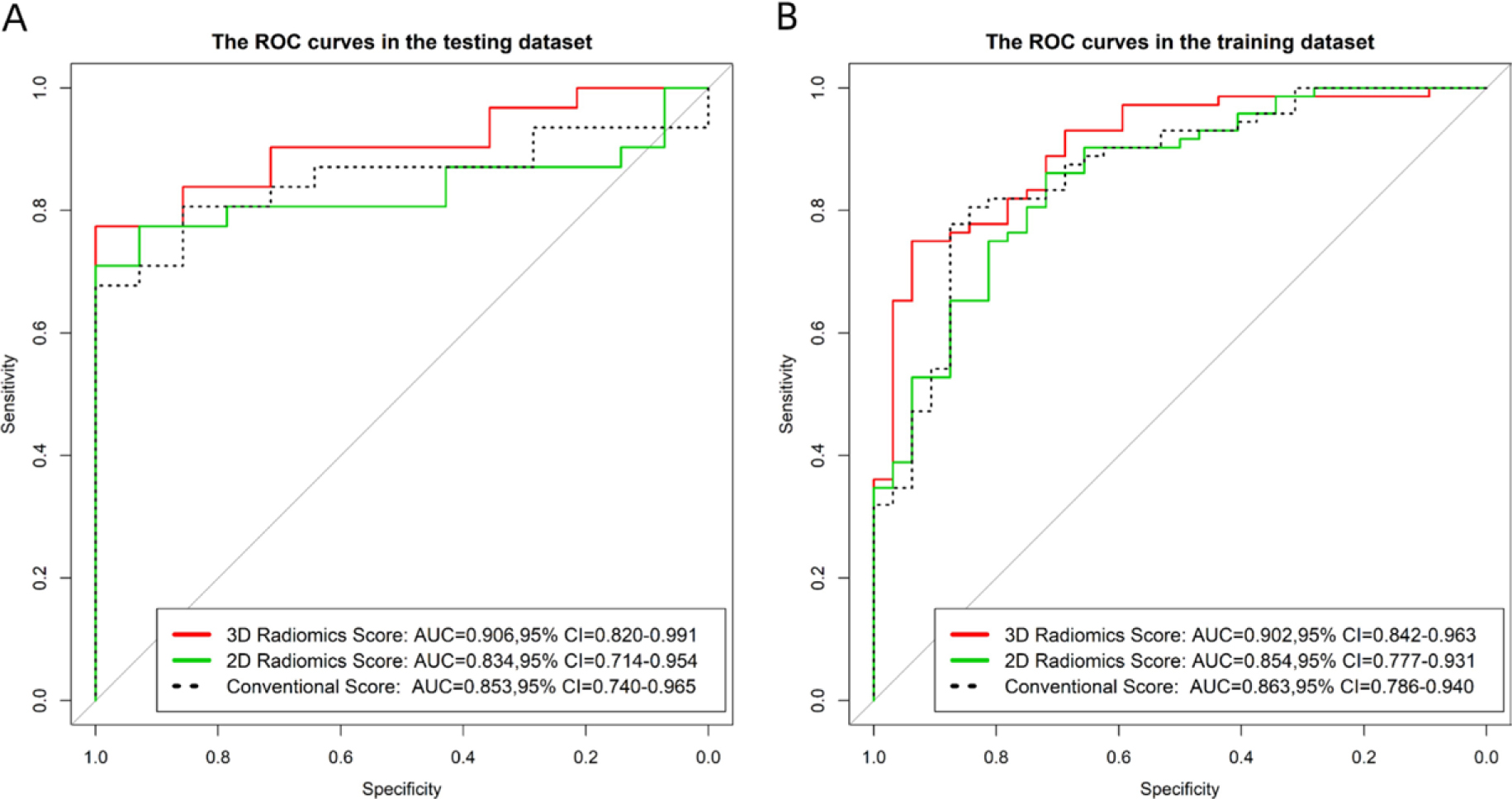
Figure 3.
Receiver operating characteristic (ROC) curve analysis of the conventional, 2D and 3D radiomics models: (A) the training set; (B) the testing set.
Table 3.
Diagnostic performance of the three models
| Model | Training dataset | Testing dataset | ||||
|---|---|---|---|---|---|---|
| Sensitivity | Specificity | AUC (95%CI) | Sensitivity | Specificity | AUC (95%CI) | |
| Conventional models | 77.8% | 87.5% | 0.863(0.786-0.940) | 54.8% | 100.0% | 0.853(0.740-0.965) |
| 2D radiomics model | 86.1% | 71.9% | 0.854(0.777-0.931) | 77.4% | 85.7% | 0.834(0.714-0.984) |
| 3D radiomics model | 75.0% | 93.8% | 0.902(0.842-0.963) | 67.7% | 100.0% | 0.906(0.820-0.991) |
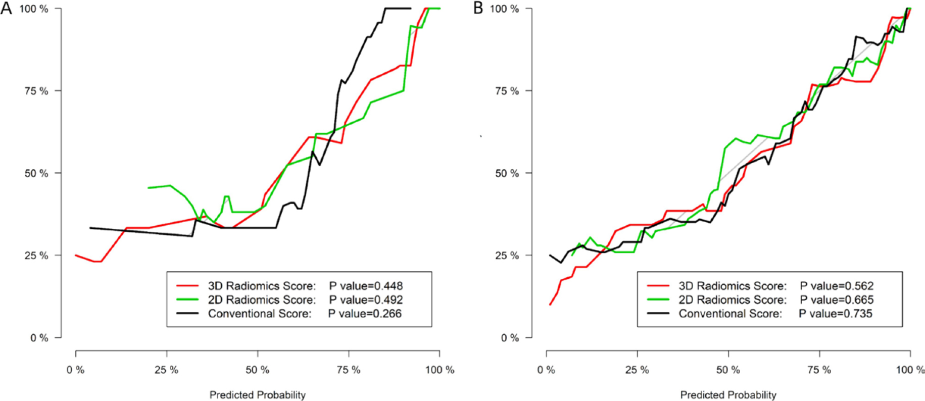
Figure 4.
The calibration curves of the conventional, 2D and 3D radiomics models:(A) the training set; (B) the testing set.
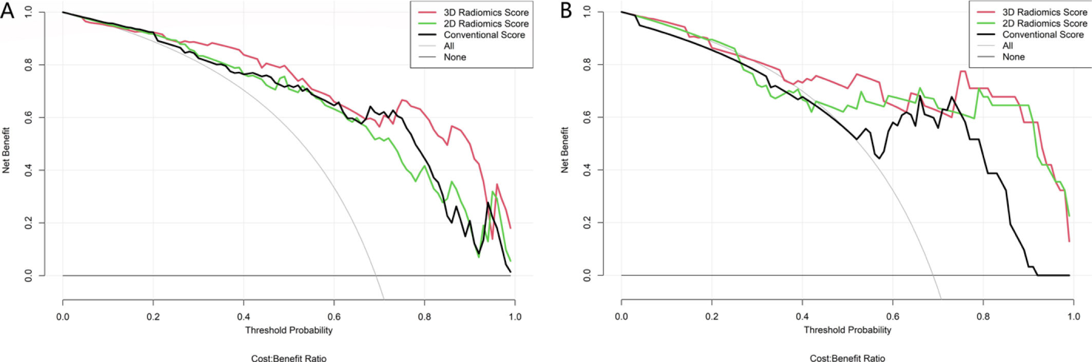
Figure 5.
Decision curve analysis (DCA) to determine the clinical usefulness of the models by quantifying the net benefits under different threshold probabilities: (A) the training set; (B) the testing set.