
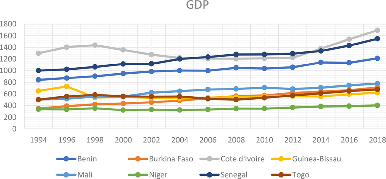
Fig. 1
GDP per capita.
Source: authors’ computation.
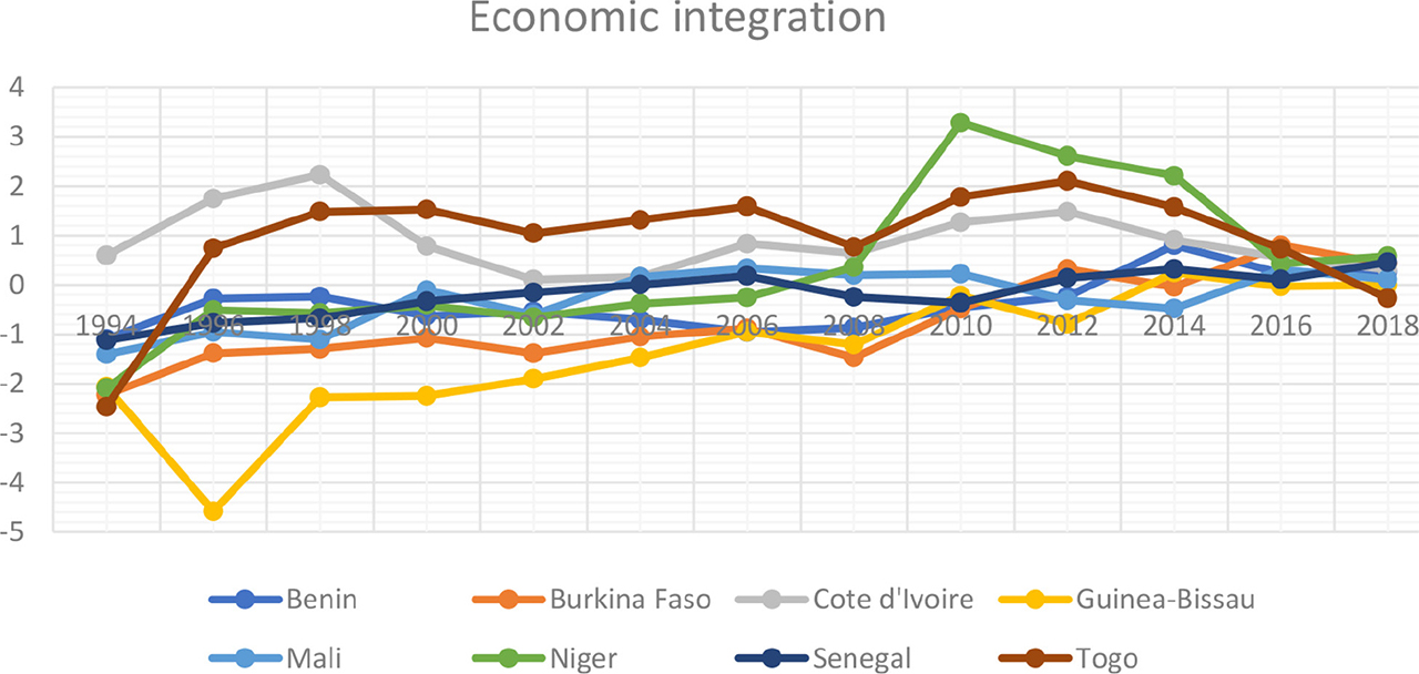
Fig. 2
Regional economic integration index.
Source: authors’ computation.
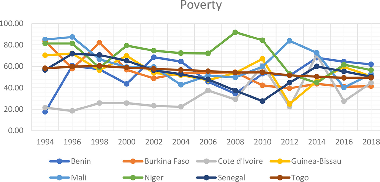
Fig. 3
Poverty headcount rate.
Source: authors’ computation.
Table 1
Definition and data sources.
| Variable name | Symbol | Definition | Unit | Source |
|---|---|---|---|---|
| Poverty | POV | It is a situation where someone lacks the necessary resource he/she needs. | % | World Development Indicators and POVCALNET |
| Income inequality | GINI | It measures the distribution of wellbeing. | Index | World Development Indicators and Standardized World Income Inequality Database (Solt 2019). |
| Remittances | REM | It is the sum of money sent by migrants to their families at home or for saving. | % | World Development Indicators |
| Control of corruption | CC | It is the extent to which public officers use public power/resource for private gain. A higher value indicates a high level of corruption. | Index | Worldwide Governance Indicators |
| Gross domestic product per capita | GDP | It is the gross domestic product divided by population. | Constant 2010 US$ | World Development Indicators |
| Population growth | POP | It is the annual growth rate of the population. | % | World Development Indicators |
| Regional economic integration | REI | It is measured with trade liberalisation (% of GDP), foreign direct investment (% of GDP), migration flow (%) and inflation rate (%, CPI). | Index | World Development Indicators, UNCTAD statistics database, United Nations Population Division |
[i] Source: authors’ compilations.
Table 2
Descriptive statistics.
| Variables | POV | GINI | REI | REM | GDP | CC | POP |
|---|---|---|---|---|---|---|---|
| Mean | 53.612 | 22.059 | 0.000 | 3.689 | 779.831 | −0.663 | 2.840 |
| Median | 54.468 | 24.288 | −0.062 | 2.559 | 648.281 | −0.676 | 2.798 |
| Maximum | 92.847 | 49.900 | 5.408 | 10.711 | 1,692.545 | 0.176 | 3.907 |
| Minimum | 10.029 | −28.100 | −4.583 | 0.226 | 322.778 | −1.563 | 1.912 |
| Std. Dev. | 16.818 | 18.421 | 1.224 | 2.823 | 351.196 | 0.381 | 0.449 |
| Skewness | −0.193 | −0.064 | 0.254 | 0.959 | 0.601 | 0.074 | 0.558 |
| Kurtosis | 2.882 | 1.311 | 5.810 | 2.712 | 2.128 | 2.541 | 3.073 |
| Jarque-Bera | 1.355 | 23.911*** | 67.976*** | 31.370*** | 18.363*** | 1.935 | 10.411*** |
| Probability | 0.508 | 0.000 | 0.000 | 0.000 | 0.000 | 0.380 | 0.005 |
Table 3
Correlation results
| POV | GINI | REI | REM | GDP | CC | POP | |
|---|---|---|---|---|---|---|---|
| POV | 1.000 | ||||||
| GINI | −0.256 | 1.000 | |||||
| REI | −0.214 | 0.239 | 1.000 | ||||
| REM | −0.070 | −0.175 | 0.222 | 1.000 | |||
| GDP | −0.486 | 0.204 | 0.147 | 0.038 | 1.000 | ||
| CC | −0.023 | 0.181 | −0.021 | −0.028 | 0.287 | 1.000 | |
| POP | 0.210 | −0.141 | 0.297 | −0.183 | −0.381 | 0.210 | 1.000 |
[i] Source: authors’ compilations.
Table 4
VIF results.
| Variables | VIF | 1/VIF |
|---|---|---|
| POP | 2.14 | 0.467 |
| REI | 1.75 | 0.572 |
| GDP | 1.68 | 0.595 |
| CC | 1.48 | 0.676 |
| GINI | 1.37 | 0.727 |
| REM | 1.34 | 0.747 |
| Mean VIF | 1.63 |
[i] Source: author's compilations.
[ii] VIF – Variance Inflation Factor.
Table 5
Cross-sectional dependence results.
Table 6
Panel unit root test results.
| Variables | CIPS | CADF | ||
|---|---|---|---|---|
| Level | First difference | Level | First difference | |
| lnPOV | −3.417*** | −5.345*** | −3.017** | −3.970*** |
| GINI | −4.849*** | −6.420*** | −3.129*** | −4.710*** |
| REI | −2.959** | −5.540*** | −2.446 | −4.277*** |
| lnREM | −1.727 | −3.885*** | −1.948 | −3.322*** |
| lnGDP | −2.142 | −4.587*** | −2.547 | −3.856*** |
| CC | −2.174 | −4.565*** | −2.031 | −3.417*** |
| POP | −4.263*** | −4.937*** | −5.180*** | −5.568*** |
| Critical values | 1%: −3.1 5%: −2.86 10%: −2.73 | 1%: −3.100 5%: −2.860 10%: −2.730 | ||
Table 7
Westerlund panel cointegration test results.
| Statistics | Value | Z-value | P value | Robust P value |
|---|---|---|---|---|
| Income distribution equation | ||||
| Gt | −30.138 | −83.323 | 0.000 | 0.000 |
| Ga | −7.610 | 3.576 | 1.000 | 0.380 |
| Pt | −42.230 | −34.492 | 0.000 | 0.000 |
| Pa | −7.164 | 2.670 | 0.996 | 0.460 |
| Poverty equation | ||||
| Gt | −4.010 | −2.560 | 0.005 | 0.010 |
| Ga | −2.350 | 5.513 | 1.000 | 1.000 |
| Pt | −10.378 | −2.035 | 0.021 | 0.020 |
| Pa | −1.986 | 4.639 | 1.000 | 0.980 |
[i] Note: A constant and a trend are used with 0 lag and 0 lead.
[ii] Source: authors’ compilations.
Table 8
PMG estimation results.
| Variables | GINI index | Poverty headcount | ||
|---|---|---|---|---|
| Coefficient | Std. err. | Coefficient | Std. err. | |
| Short run | ||||
| ECT | −0.760*** | 0.131 | 0.0697 | 0.0971 |
| ΔlnPOV(−1) | – | – | 0.510*** | 0.0369 |
| ΔREI | −0.176 | 0.137 | 0.162 | 0.121 |
| ΔEI(−1) | −0.129 | 0.0993 | ||
| ΔGINI | – | – | −0.0191 | 0.0354 |
| ΔGINI(−1) | – | – | 0.0138 | 0.0174 |
| ΔlnREM | −0.470 | 0.487 | −0.263 | 0.171 |
| ΔlnREM(−1) | – | – | 0.338 | 0.222 |
| ΔlnGDP | 45.44** | 20.92 | −1.456 | 1.114 |
| ΔCC | 1.509** | 0.695 | 0.0910 | 0.194 |
| ΔPOP | 9.780 | 8.824 | −0.880 | 0.702 |
| ΔPOP (−1) | – | – | 0.931 | 1.396 |
| Constant | 9.221** | 4.700 | 0.128 | 0.108 |
| Long run | ||||
| REI | 0.0684* | 0.0367 | −0.0761*** | 0.0224 |
| GINI | – | – | −0.0475*** | 0.0111 |
| lnREM | −0.0308 | 0.059 | 0.172*** | 0.0439 |
| lnGDP | 0.138 | 0.211 | 0.549*** | 0.204 |
| CC | −0.0804 | 0.154 | 0.126** | 0.0643 |
| POP | 0.753*** | 0.132 | 1.136*** | 0.213 |
| Number of observation | 192 | 184 | ||
Table 9
Time-series analysis results based on the DOLS method.
| Countries | Benin | Burkina Faso | Côte d’Ivoire | Guinea-Bissau | Mali | Niger | Senegal | Togo | ||||||||
|---|---|---|---|---|---|---|---|---|---|---|---|---|---|---|---|---|
| GINI | POV | GINI | POV | GINI | POV | GINI | POV | GINI | POV | GINI | POV | GINI | POV | GINI | POV | |
| REI | 21.72*** (0.404) | −0.410*** (0.0778) | 13.70*** (0.504) | −0.0439 (0.0610) | 37.51*** (0.218) | 8.256*** (0.0426) | −27.39*** (1.284) | −1.738*** (0.0427) | −20.88*** (0.639) | 3.868*** (0.0848) | −4.117*** (0.331) | −0.0763*** (0.0125) | −6.574*** (0.773) | 4.694*** (0.0930) | 0.889*** (0.0629) | 0.0473*** (0.00293) |
| GINI | – | 0.434*** (0.0261) | – | 0.0161 (0.0101) | – | −0.0378** (0.0158) | – | 0.0118*** (0.00398) | – | −0.0750*** (0.00875) | – | 0.210*** (0.00354) | – | 0.961*** (0.0101) | – | −0.0615*** (0.00318) |
| lnREM | 3.935*** (0.574) | 0.430*** (0.131) | −25.24*** (0.729) | 0.490*** (0.0755) | −11.50*** (1.060) | −9.812*** (0.217) | 47.94*** (1.891) | 3.426*** (0.0643) | 524.8*** (0.886) | −2.416*** (0.128) | −18.06*** (1.013) | 0.452*** (0.0384) | −16.40*** (0.710) | −14.39*** (0.0851) | −0.405*** (0.130) | 0.246*** (0.00541) |
| lnGDP | −336.6*** (4.239) | −5.705*** (0.952) | 11.89*** (2.466) | −1.061*** (0.258) | 96.68*** (2.409) | 4.606*** (0.470) | 180.7*** (11.51) | −0.817* (0.429) | −1,490*** (3.473) | −0.0993 (0.507) | 13.76** (6.074) | −1.598*** (0.248) | 82.09*** (3.111) | −3.765*** (0.383) | 16.14*** (1.195) | 0.421*** (0.0520) |
| CC | 82.29*** (1.202) | −1.150*** (0.235) | −1.217 (2.310) | 1.367*** (0.243) | 16.78*** (0.995) | 4.571*** (0.192) | 110.2*** (6.415) | 5.054*** (0.214) | 451.2*** (2.953) | −1.850*** (0.383) | 42.24*** (3.598) | −3.687*** (0.138) | 12.12*** (0.726) | −8.876*** (0.0846) | 9.481*** (0.951) | 0.00849 (0.0399) |
| POP | −152.2*** (1.578) | 9.313*** (0.306) | −186.1*** (7.143) | 5.575*** (0.770) | −106.6*** (0.722) | −12.98*** (0.138) | 56.74*** (5.049) | 3.464*** (0.181) | −566.3*** (1.891) | 2.314*** (0.252) | 51.68*** (6.414) | 2.547*** (0.244) | 1.946* (1.087) | 20.10*** (0.133) | 6.701*** (0.332) | 1.271*** (0.0142) |
Table 10
Heterogeneous panel causality test results.
| lnPOV | GINI | REI | lnREM | lnGDP | CC | POP | |
|---|---|---|---|---|---|---|---|
| lnPOV | −0.5599 (0.5756) | 2.0470** (0.0407) | 0.4123 (0.6801) | 1.1441 (0.2526) | −0.3039 (0.7612) | 0.6270 (0.5307) | |
| GINI | 0.6428 (0.5204) | −0.4899 (0.6242) | 0.8665 (0.3862) | 0.3513 (0.7254) | −0.6080 (0.5432) | −0.1381 (0.8902) | |
| REI | 3.1594*** (0.0016) | 2.7527*** (0.0059) | 3.8692*** (0.0000) | 0.5314 (0.5951) | −0.5156 (0.6061) | 0.9304 (0.3522) | |
| lnREM | 2.7370*** (0.0062) | 0.9483 (0.3430) | 2.2553** (0.0241) | 2.6512*** (0.0080) | 3.2922*** (0.0010) | −0.1016 (0.9191) | |
| lnGDP | 2.3861** (0.0170) | 0.9317*** (0.0000) | 2.5827*** (0.0098) | 2.8435*** (0.0045) | −0.1012 (0.9033) | 2.7147*** (0.0066) | |
| CC | −0.5047 (0.6138) | 2.9592*** (0.0031) | 1.6822* (0.0925) | 2.2788** (0.0227) | 1.8482* (0.0646) | 1.2308 (0.2184) | |
| POP | 6.2131*** (0.0000) | 3.6573*** (0.0003) | 2.7282*** (0.0064) | 4.6874*** (0.0000) | 2.7159*** (0.0066) | 2.2000** (0.0278) |
Table 11
Principal component analysis details.
| Number | Value | Difference | Proportion | Cumulative value | Cumulative proportion |
|---|---|---|---|---|---|
| Panel A: Eigen values of the observed matrix | |||||
| 1 | 1.491 | 0.490 | 0.373 | 1.491 | 0.373 |
| 2 | 1.001 | 0.171 | 0.250 | 2.492 | 0.623 |
| 3 | 0.831 | 0.153 | 0.208 | 3.323 | 0.831 |
| 4 | 0.677 | – | 0.169 | 4.000 | 1.000 |
| Panel B: Eigenvectors (loadings) | |||||
| Variable | PC1 | PC2 | PC3 | PC4 | |
| REI1 | 0.558 | 0.448 | 0.173 | −0.677 | |
| REI2 | 0.550 | 0.398 | −0.404 | 0.613 | |
| REI3 | 0.483 | −0.416 | 0.708 | 0.304 | |
| REI4 | −0.391 | 0.684 | 0.552 | 0.272 | |
| Panel C: Ordinary correlations | |||||
| REI1 | REI2 | REI3 | REI4 | ||
| REI1 | 1.000 | ||||
| REI2 | 0.297 | 1.000 | |||
| REI3 | 0.178 | 0.119 | 1.000 | ||
| REI4 | −0.064 | −0.121 | −0.186 | 1.000 | |
[i] Source: authors’ compilations.