
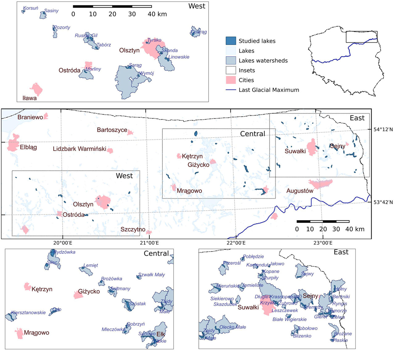
Fig. 1
Location of lakes and extent of the watershed on the study area.
Table 1
Explanatory variables used in the study.
| Variable | Abbreviation | Unit | Source |
|---|---|---|---|
| Elevation | ELEV | m a.s.l. | Jańczak 1999 |
| Lake area | LARE | ha | Jańczak 1999 |
| Lake capacity | LCAP | km3 | Jańczak 1999 |
| Lake max depth | LDMX | m | Jańczak 1999 |
| Lake average depth | LDAV | m | Jańczak 1999 |
| Lake max length | LLEN | m | Jańczak 1999 |
| Lake max width | LWID | m | Jańczak 1999 |
| Lake shoreline length | PRIM | m | Jańczak 1999 |
| Lake elongation | LELN | Ratio | LLEN / LW ID |
| Lake capacity/length ratio | LVAR | Ratio | LCAP / LLEN |
| Lake perim development | LPDV | Ratio | LLEN / sqrt (2 × π × LARE) |
| Lake exposition | LEXP | Ratio | LARE / LDAV |
| Watershed area | WARE | ha | Calculated |
| Mean slope | WSLP | % | Calculated |
| Height stddev | WHSD | m | Calculated |
| Urbanised | WURB | % | Calculated |
| Agriculture | WAGR | % | Calculated |
| Forests | WFRS | % | Calculated |
| Wetlands | WWET | % | Calculated |
| Sands | WSND | % | Calculated |
| Tills | WTLS | % | Calculated |
| Clay | WCLS | % | Calculated |
| Organic | WORG | % | Calculated |
| Schindler ratio | SR | Ratio | WARE / LCAP |
| Ohle ratio | OR | Ratio | WARE / LARE |
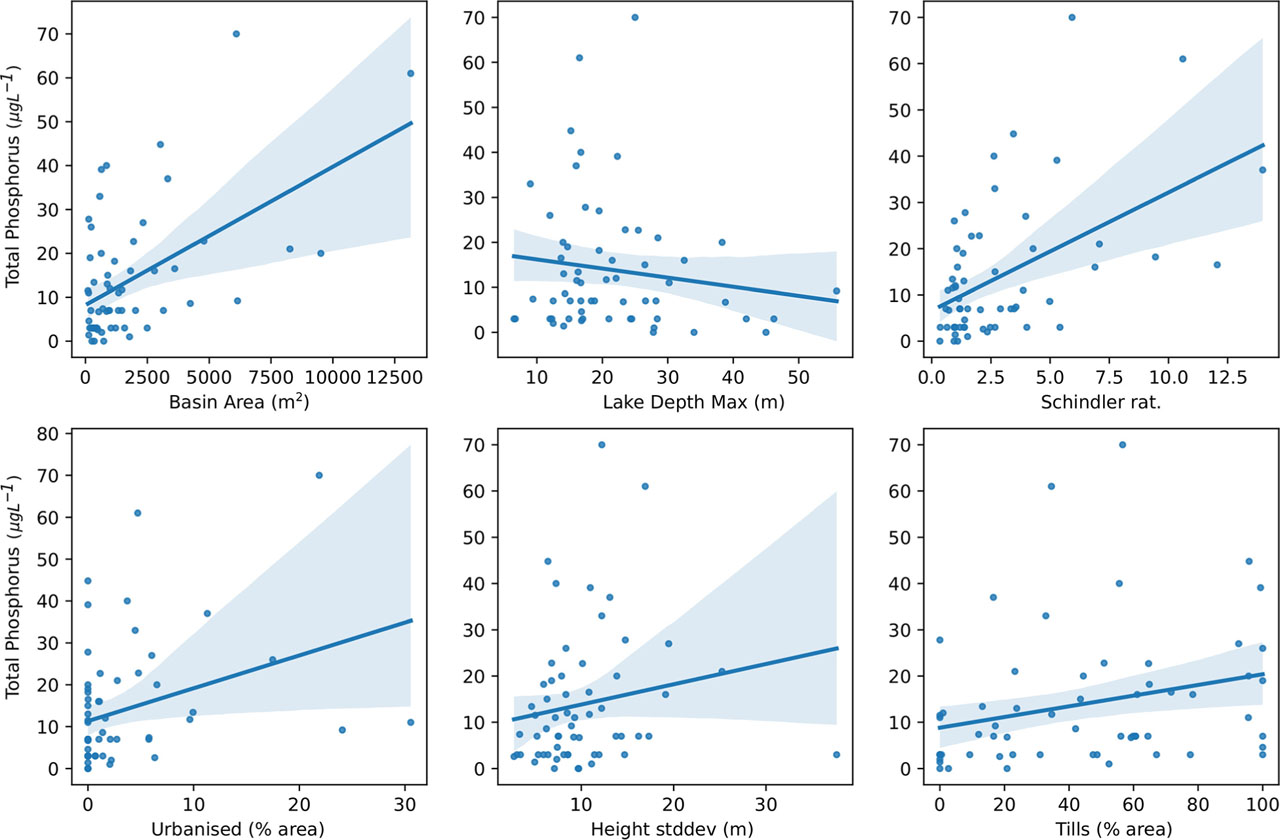
Fig. 2
Relations between Ptot and selected explanatory variables, see Table 1 for details.
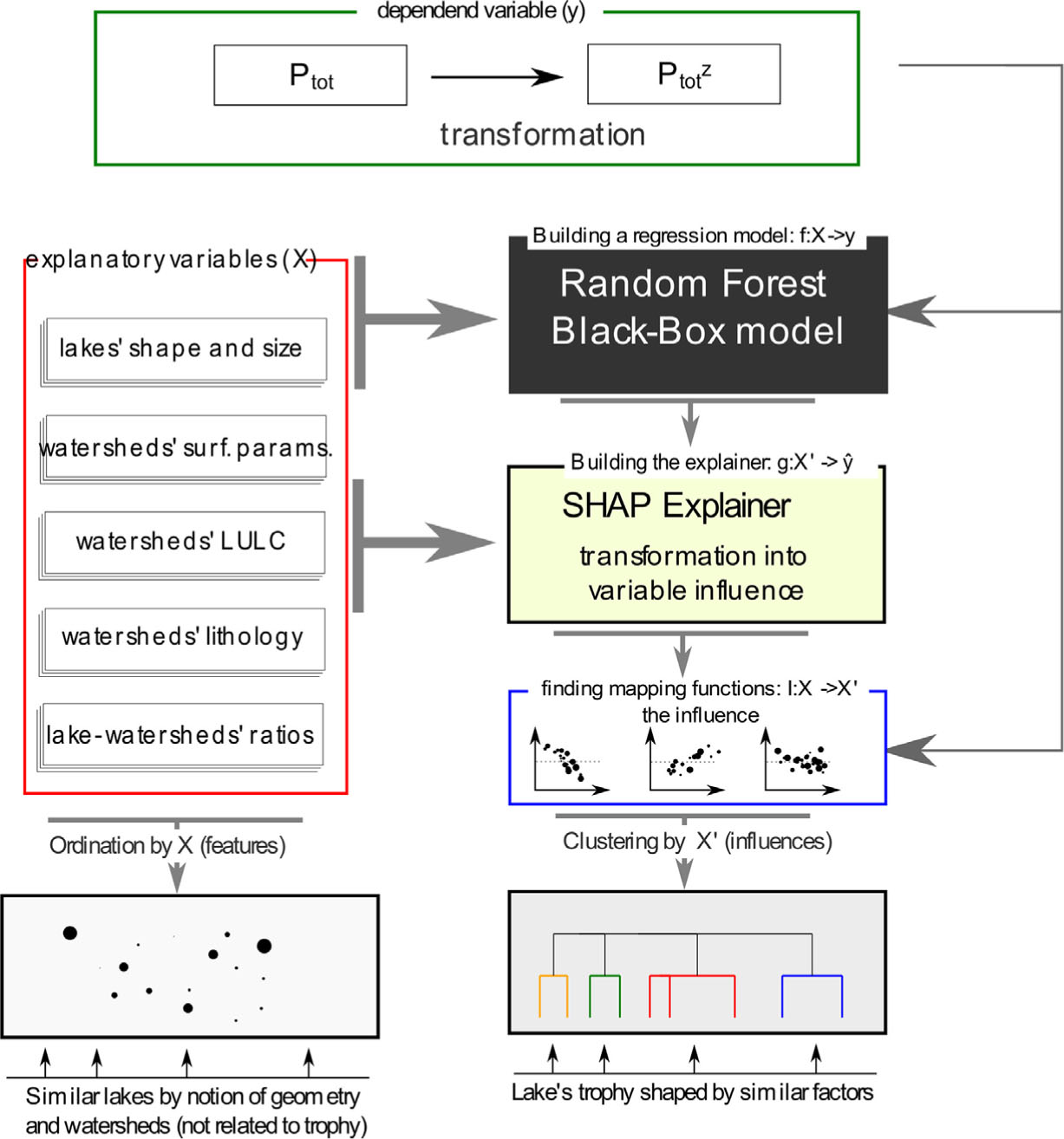
Fig. 3
The outline of methodology. See Section ‘Methods’ for details.
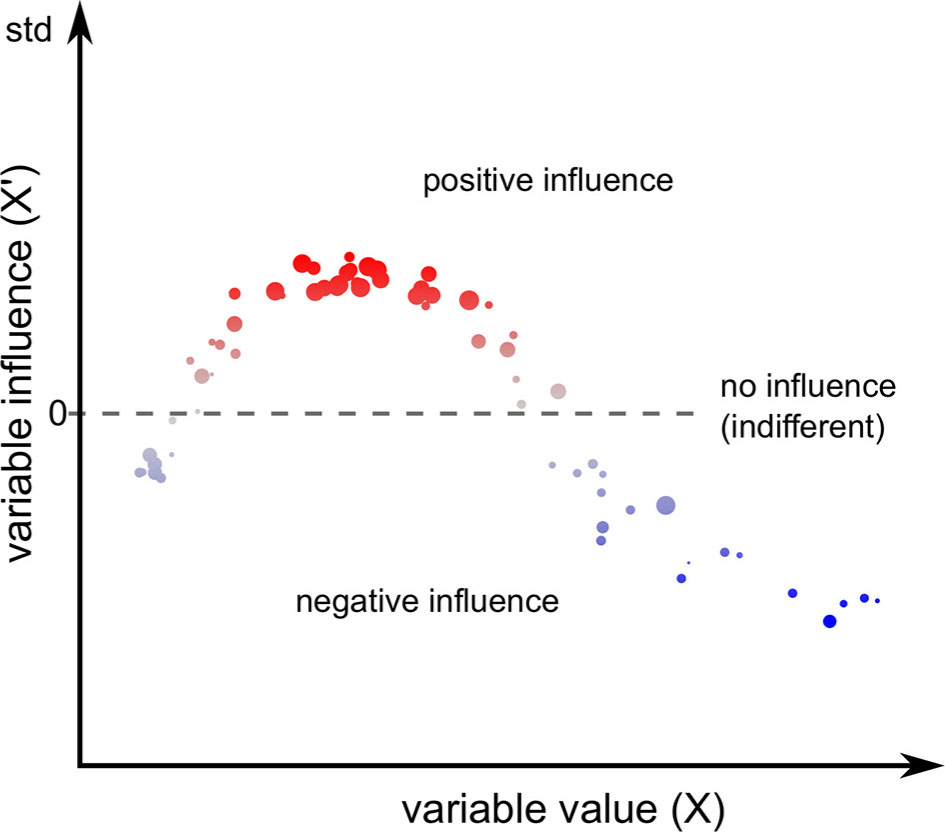
Fig. 4
The concept of mapping variable values into influence. The size of dots simulates the values of the dependent variable.
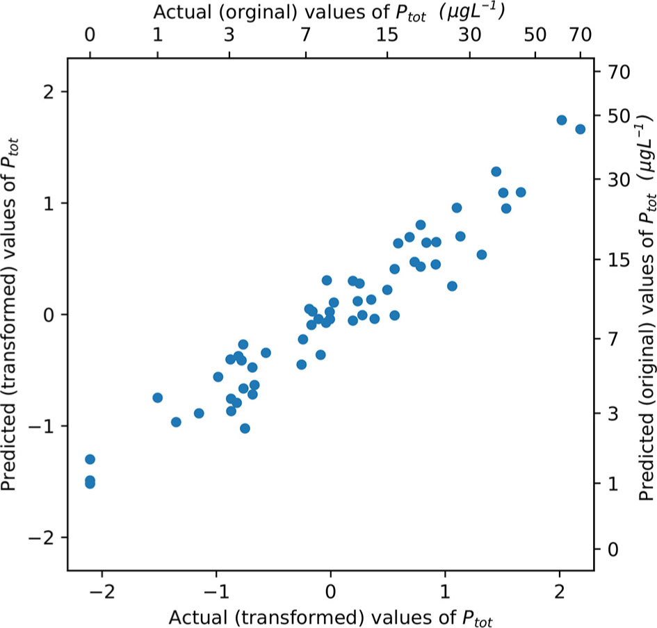
Fig. 5
Relation between actual values of dependent variables and the outcome of the model Ptot.
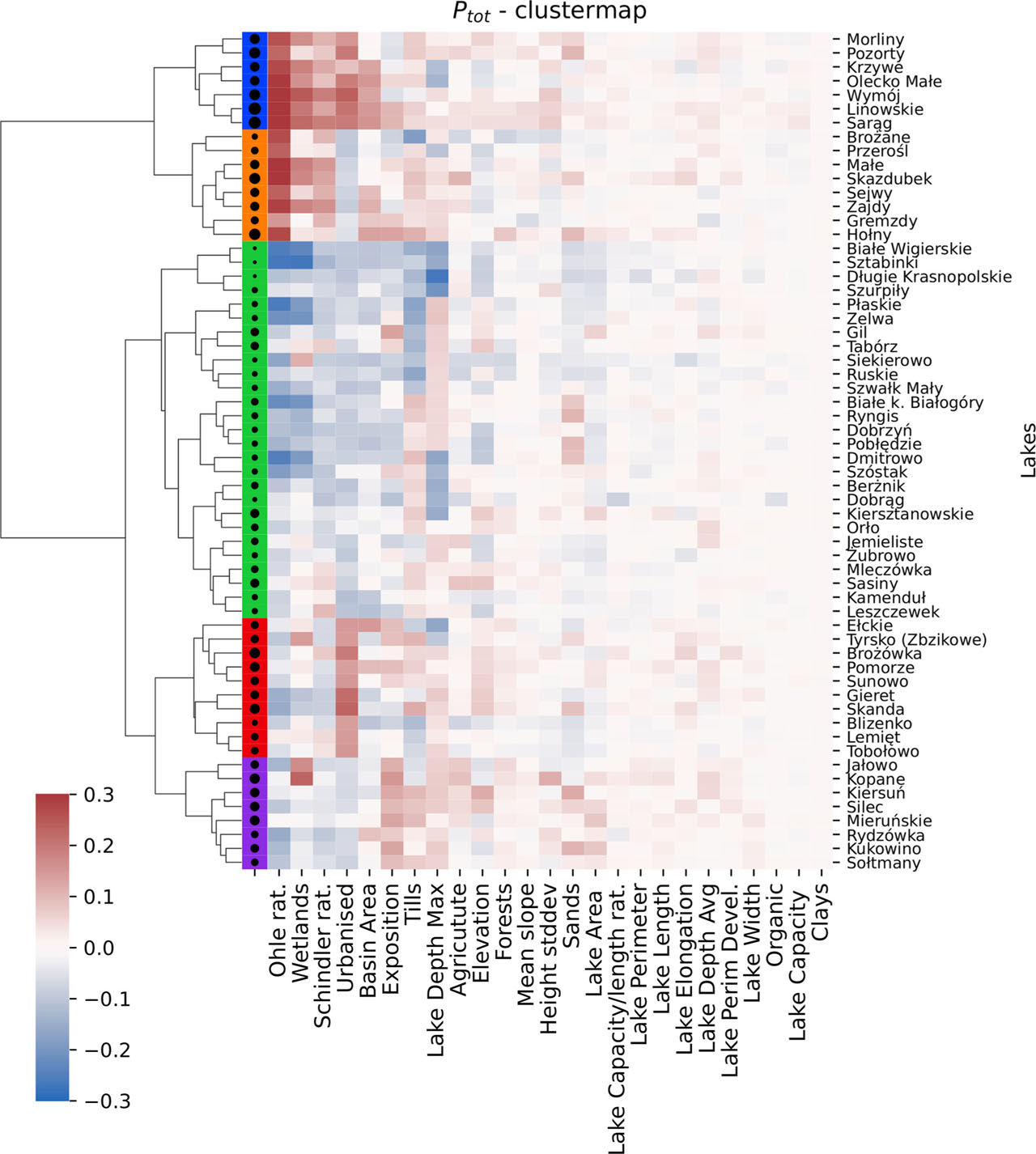
Fig. 6
Relation between clusters and variable influence. The red-white-blue gradient denotes the influence of the given variable. The colours marking the clusters are used in the same way in the other figures.
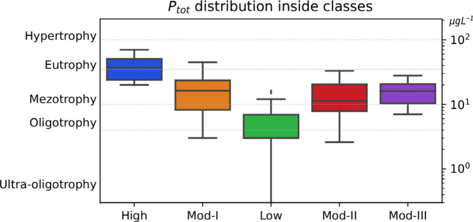
Fig. 7
Variation of Ptot in clusters. X-labels denote the name of the class: High trophy, Moderate trophy (Mod.-I, Mod.-II, Mod.-III), and Low trophy.
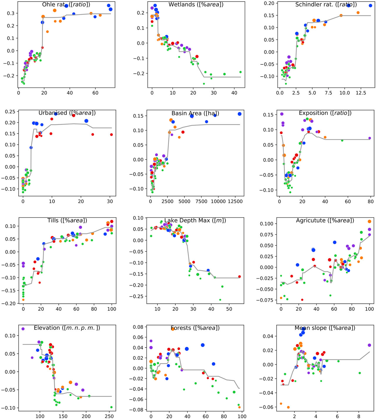
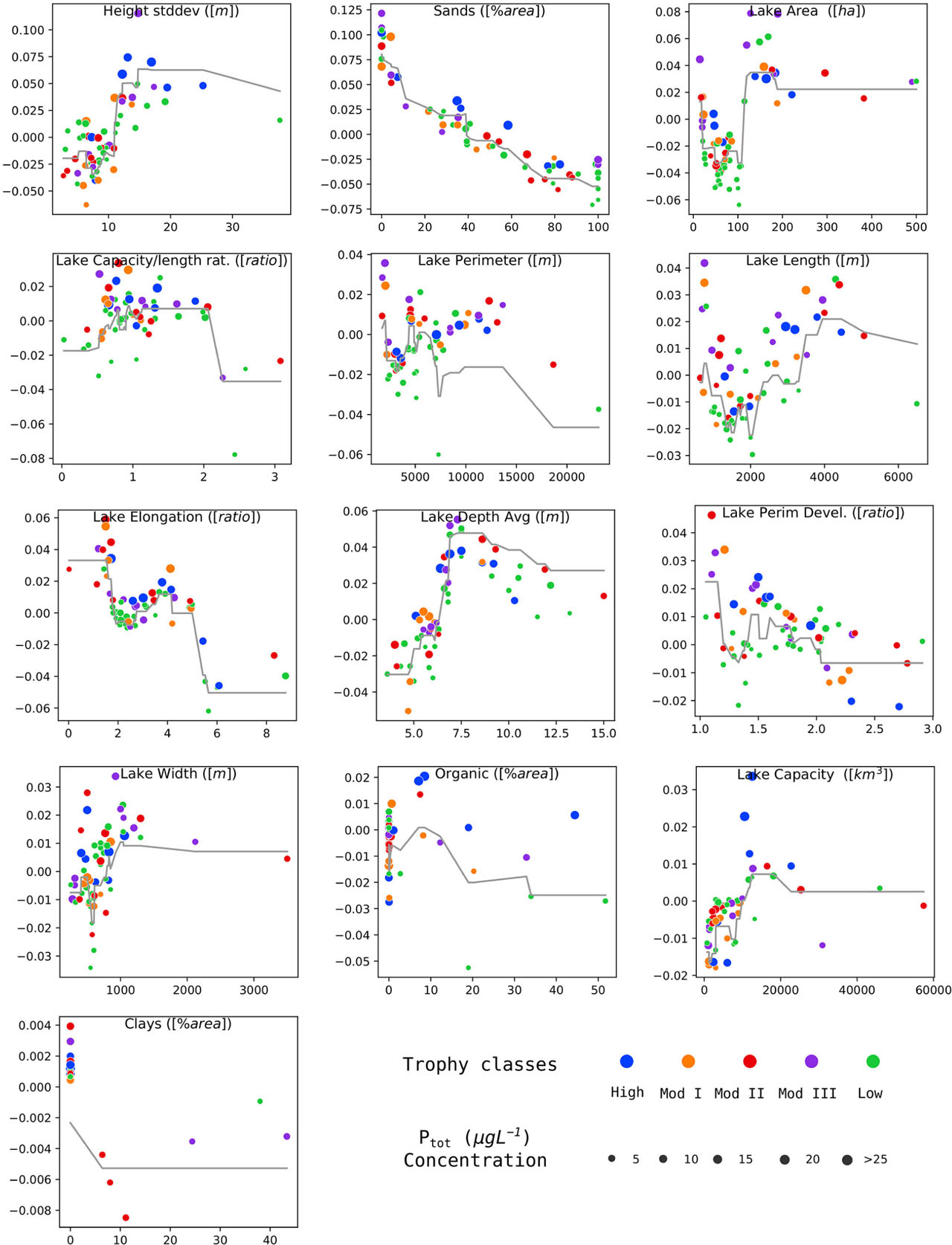
Fig. 8
The influence plots for each variable. The X-axis contains the original values of the variable, Y-axis contains the influence. Colours in legend denote clusters (see Fig. 7), size of dots value of Ptot. Partial Dependency Plot (PDP) is marked by a light grey line.
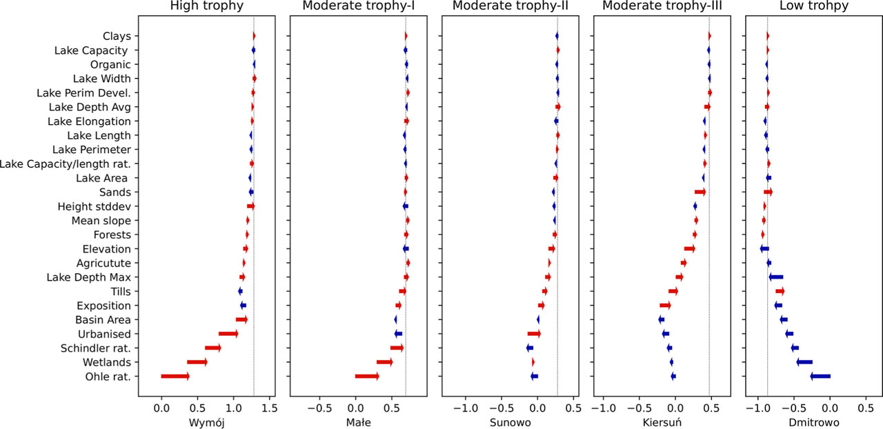
Fig. 9
The SHAP (SHapley Additive exPlanations) plots (Lundberg, Lee 2017) for the five most representative lakes for each class. X-axis presents influence in units of Ptot standard deviation scale is the same for each subplot, but ranges are different. Length and direction of arrows denote the scale and influence orientation (negative or positive) brought by a given variable.
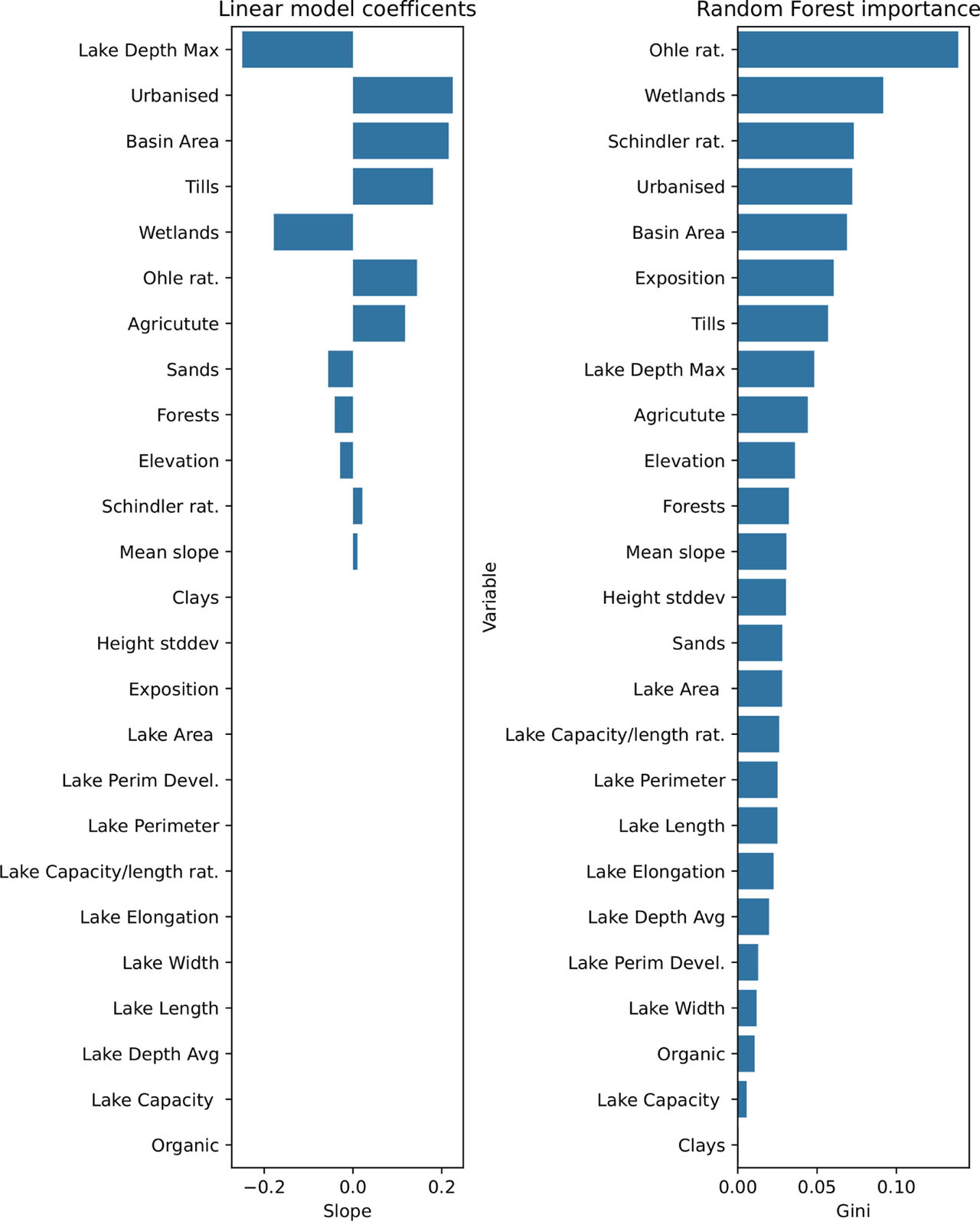
Fig. 10
The variable importance estimated using multiple linear regression (ElasticNet) and random forest. See text for details.
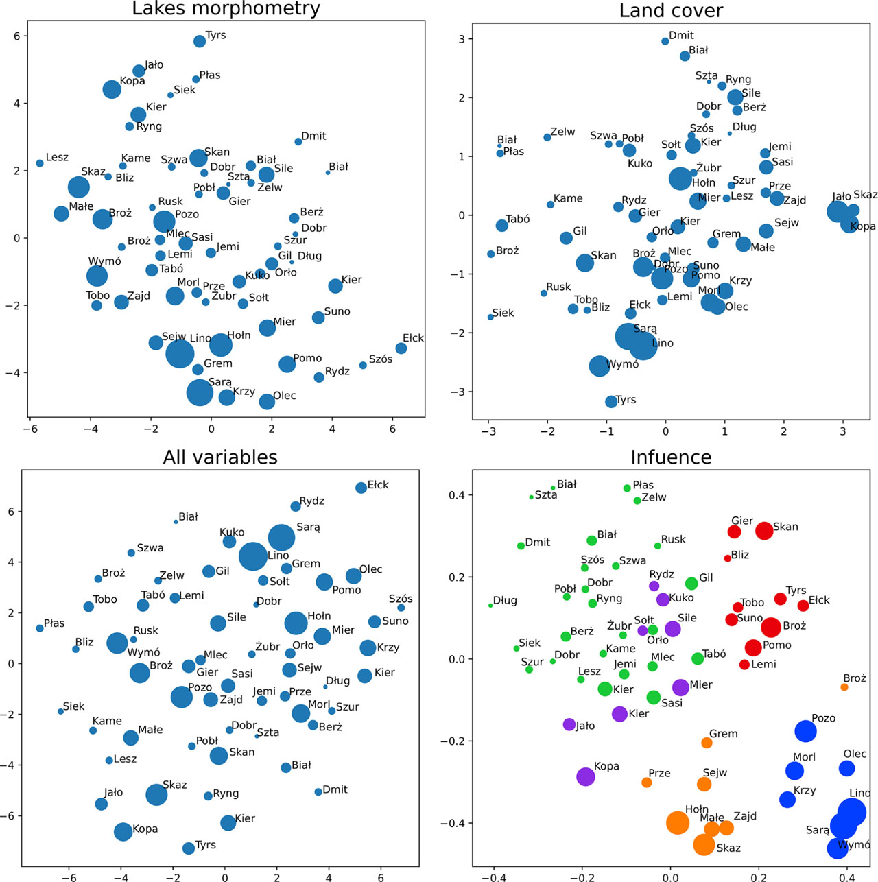
Fig. 11
Visualisation of dissimilarities between lakes in a form of MDS (multidimensional scaling). The axes of the plot have no units. Lakes morphometry presents dissimilarity for a group of morphometric features (see Table 1); Land cover presents dissimilarity for four land cover variables (urbanised, agriculture, forests, wetlands); ‘All variables’ plate uses all 25 variables; Influence presents dissimilarity between lakes in a space of variables influence. For colours see Figure 7.