
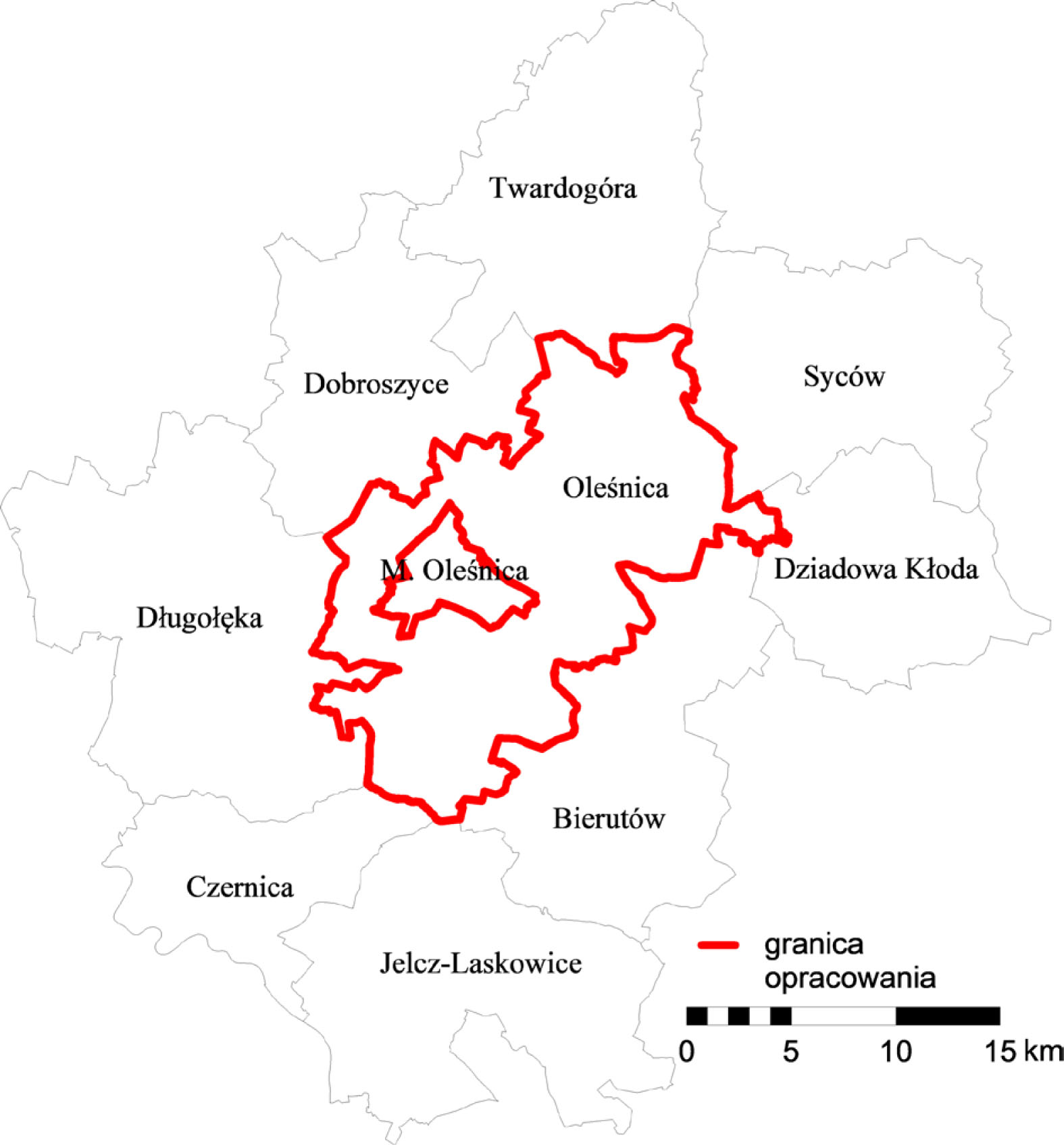
Fig. 1
Study area – as of 2016.
Source: own study.
Table 1
Compatibility matrix of land use allocations.
| MN | MW | U | US | UC | U/P | MN/U | MW/U | R | RU | RM | P | PG | ZN | ZL | ZP | ZD | ZC | WS | KD | TK | TZ | KL | |
|---|---|---|---|---|---|---|---|---|---|---|---|---|---|---|---|---|---|---|---|---|---|---|---|
| MN | 0 | 0 | 1 | 0 | 1 | 2 | 0 | 0 | 2 | 2 | 2 | 2 | 2 | 2 | 1 | 0 | 2 | 1 | 1 | 1 | 1 | 1 | 1 |
| MW | 0 | 0 | 1 | 0 | 1 | 2 | 0 | 0 | 2 | 2 | 2 | 2 | 2 | 2 | 1 | 0 | 2 | 1 | 1 | 1 | 1 | 1 | 1 |
| U | 1 | 1 | 0 | 1 | 0 | 0 | 1 | 1 | 1 | 1 | 1 | 0 | 0 | 2 | 1 | 1 | 1 | 1 | 1 | 0 | 0 | 1 | 0 |
| US | 0 | 0 | 1 | 0 | 1 | 2 | 0 | 0 | 2 | 2 | 2 | 2 | 2 | 1 | 2 | 0 | 2 | 1 | 0 | 1 | 0 | 1 | 1 |
| UC | 1 | 1 | 0 | 1 | 0 | 0 | 1 | 1 | 1 | 1 | 1 | 0 | 1 | 2 | 1 | 1 | 1 | 1 | 1 | 0 | 0 | 1 | 0 |
| U/P | 2 | 2 | 0 | 2 | 0 | 0 | 2 | 2 | 2 | 2 | 2 | 0 | 0 | 2 | 2 | 1 | 2 | 1 | 1 | 0 | 0 | 1 | 0 |
| MN/U | 0 | 0 | 1 | 0 | 1 | 2 | 0 | 0 | 1 | 1 | 2 | 2 | 2 | 2 | 1 | 0 | 2 | 1 | 1 | 1 | 1 | 1 | 1 |
| MW/U | 0 | 0 | 1 | 0 | 1 | 2 | 0 | 0 | 2 | 2 | 2 | 2 | 2 | 2 | 1 | 0 | 2 | 1 | 1 | 1 | 1 | 1 | 1 |
| R | 2 | 2 | 1 | 2 | 1 | 2 | 2 | 2 | 0 | 0 | 0 | 2 | 2 | 0 | 0 | 0 | 0 | 0 | 0 | 1 | 0 | 0 | 0 |
| RU | 2 | 2 | 1 | 2 | 1 | 2 | 2 | 2 | 0 | 0 | 0 | 2 | 2 | 1 | 0 | 1 | 0 | 1 | 1 | 1 | 0 | 1 | 1 |
| RM | 2 | 2 | 1 | 2 | 1 | 2 | 2 | 2 | 0 | 0 | 0 | 2 | 2 | 1 | 0 | 0 | 0 | 1 | 1 | 1 | 0 | 1 | 1 |
| P | 2 | 2 | 0 | 2 | 0 | 0 | 2 | 2 | 2 | 2 | 2 | 0 | 0 | 2 | 2 | 1 | 2 | 1 | 1 | 0 | 0 | 1 | 1 |
| PG | 2 | 2 | 0 | 2 | 1 | 0 | 2 | 2 | 2 | 2 | 2 | 0 | 0 | 1 | 2 | 1 | 2 | 1 | 1 | 0 | 0 | 1 | 1 |
| ZN | 2 | 2 | 2 | 1 | 2 | 2 | 2 | 2 | 0 | 1 | 1 | 2 | 1 | 0 | 0 | 0 | 0 | 0 | 0 | 1 | 1 | 0 | 1 |
| ZL | 1 | 1 | 1 | 1 | 1 | 1 | 1 | 1 | 0 | 0 | 0 | 2 | 2 | 0 | 0 | 0 | 0 | 0 | 0 | 1 | 0 | 0 | 1 |
| ZP | 0 | 0 | 1 | 0 | 1 | 1 | 0 | 0 | 0 | 1 | 0 | 1 | 1 | 0 | 0 | 0 | 0 | 0 | 0 | 1 | 0 | 1 | 0 |
| ZD | 2 | 2 | 1 | 2 | 1 | 2 | 2 | 2 | 0 | 0 | 0 | 2 | 2 | 0 | 0 | 0 | 0 | 0 | 0 | 1 | 0 | 1 | 0 |
| ZC | 1 | 1 | 1 | 1 | 1 | 1 | 1 | 1 | 1 | 1 | 1 | 1 | 1 | 0 | 0 | 0 | 0 | 0 | 1 | 0 | 0 | 1 | 1 |
| WS | 1 | 1 | 1 | 0 | 1 | 1 | 1 | 1 | 0 | 1 | 0 | 1 | 1 | 0 | 0 | 0 | 0 | 1 | 0 | 0 | 0 | 0 | 0 |
| KD | 1 | 1 | 0 | 1 | 0 | 0 | 1 | 1 | 1 | 1 | 1 | 0 | 0 | 1 | 1 | 1 | 1 | 0 | 0 | 0 | 0 | 0 | 0 |
| TK | 1 | 1 | 0 | 0 | 0 | 0 | 1 | 1 | 0 | 0 | 0 | 0 | 0 | 1 | 0 | 0 | 0 | 0 | 0 | 0 | 0 | 0 | 0 |
| TZ | 1 | 1 | 1 | 1 | 1 | 1 | 1 | 1 | 1 | 0 | 1 | 1 | 1 | 1 | 0 | 0 | 1 | 1 | 1 | 0 | 0 | 0 | 0 |
| KL | 1 | 1 | 0 | 1 | 0 | 0 | 1 | 1 | 0 | 1 | 1 | 1 | 1 | 1 | 1 | 0 | 0 | 1 | 0 | 0 | 0 | 0 | 0 |
[i] Source: Grochowska 2016: 52–53.
[ii] Abbreviations used in the matrix: MN – Single-family residential development areas, MW – Multi-family residential development areas, U – Service development areas, US – Sports and recreation areas, UC – Areas for commercial facilities with retail space over 2,000 m2, U/P – Service and production development areas, MN/U – Residential and service development areas, MW/U – , R – Farming areas, RU – Production service areas for arable land, livestock. Horticultural and fishing farms, RM – Homestead development areas in arable land, livestock and horticultural farms, P – Production facility, warehouse and storage areas, PG – Mining areas and lands, ZN – Uncontrolled greenery areas, ZL – Forests, ZP – Controlled greenery areas, ZD – Allotment garden areas, ZC – Cemeteries, WS – Surface water areas, KD – Road areas, TK – Railway lines and areas, TZ – Closed areas, KL – Civilian airport areas.
Table 2
Number of incompatible sections in border areas.
| No. | Communes rural (r), urban (u), urban-rural (ur) | Number of connected sections with different functions | Number of incompatible sections (SUiKZP) | Number of incompatible sections (actual development) |
|---|---|---|---|---|
| 1 | Oleśnica (r) – Oleśnica (u) | 61 | 36 | 7 |
| 2 | Oleśnica (r) – Długołęka (r) | 48 | 10 | 2 |
| 3 | Oleśnica (r) – Dobroszyce (r) | 37 | 10 | 5 |
| 4 | Oleśnica (r) – Bierutów (ur) | 36 | 7 | 0 |
| 5 | Oleśnica (r) – Syców (ur) | 35 | 9 | 1 |
| 6 | Oleśnica (r) – Twardogóra (ur) | 15 | 5 | 3 |
| 7 | Oleśnica (r) – Dziadowa-Kłoda (r) | 10 | 0 | 0 |
| 8 | Oleśnica (r) – Czernica (r) | 9 | 1 | 0 |
| 9 | Oleśnica (r) – Jelcz-Laskowice (ur) | 4 | 1 | 0 |
| Total | 255 | 79 | 18 | |
[i] Source: own study.
Table 3
Number of sections of consistent and inconsistent actual land use planning.
| No. | Communes rural (r), urban (u), urban-rural (ur) | Number of segments of different functions connected | Is the real development consistent with the intended use of the land? | |
|---|---|---|---|---|
| Yes | No | |||
| 1 | Oleśnica (r) | 255 | 200 | 55 |
| 2 | Oleśnica (u) | 61 | 30 | 31 |
| 3 | Długołęka (r) | 48 | 40 | 8 |
| 4 | Dobroszyce (r) | 37 | 32 | 5 |
| 5 | Bierutów (ur) | 36 | 30 | 6 |
| 6 | Syców (ur) | 35 | 32 | 3 |
| 7 | Twardogóra (ur) | 15 | 9 | 6 |
| 8 | Dziadowa-Kłoda (r) | 10 | 10 | 0 |
| 9 | Czernica (r) | 9 | 9 | 0 |
| 10 | Jelcz-Laskowice (ur) | 4 | 3 | 1 |
| Total | 510 | 395 | 115 | |
[i] Source: own study.
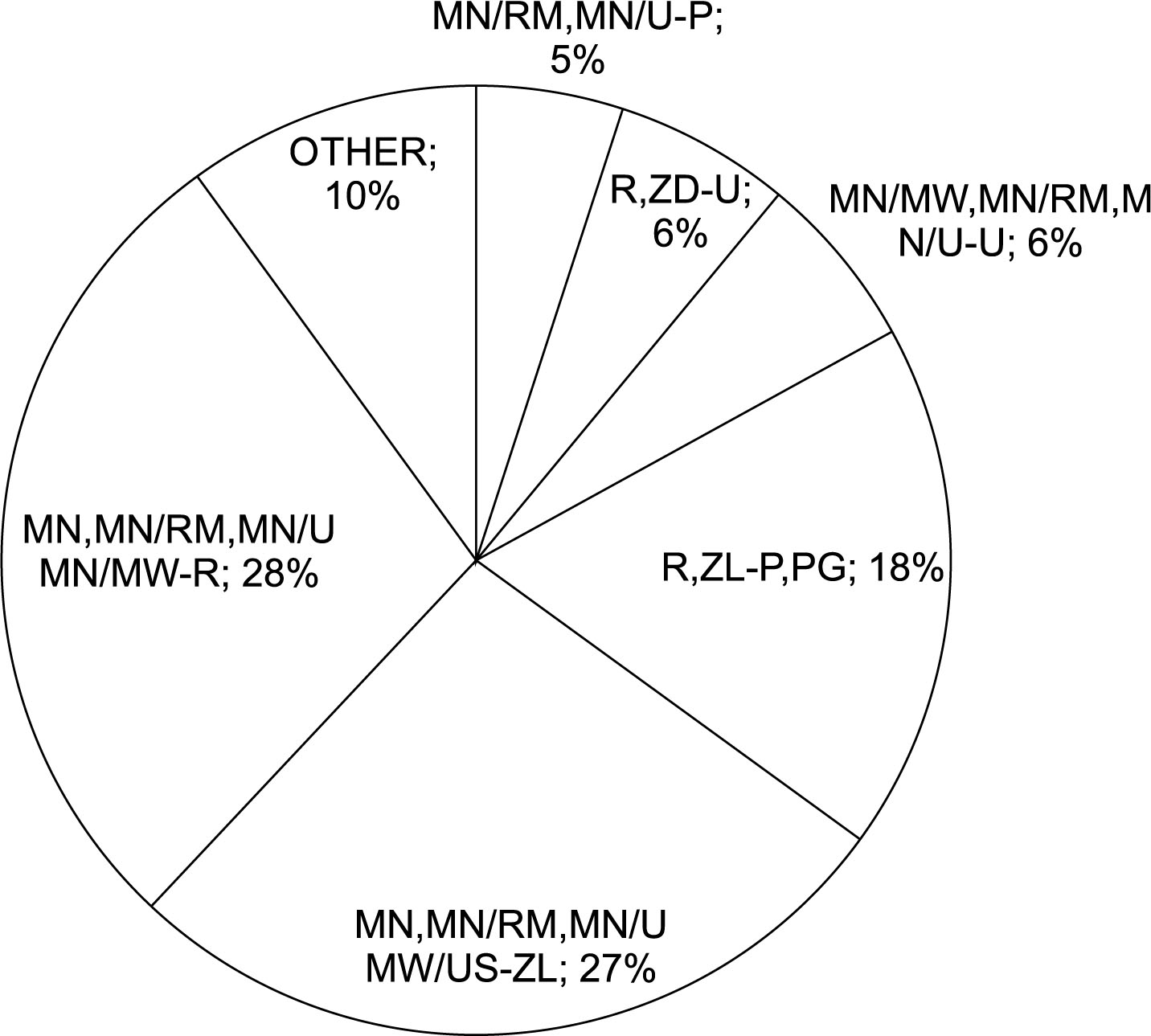
Fig. 2
Share of incompatibilities of land use allocations occurring on the border of the commune. Oleśnica – 2016.
Source: own study.
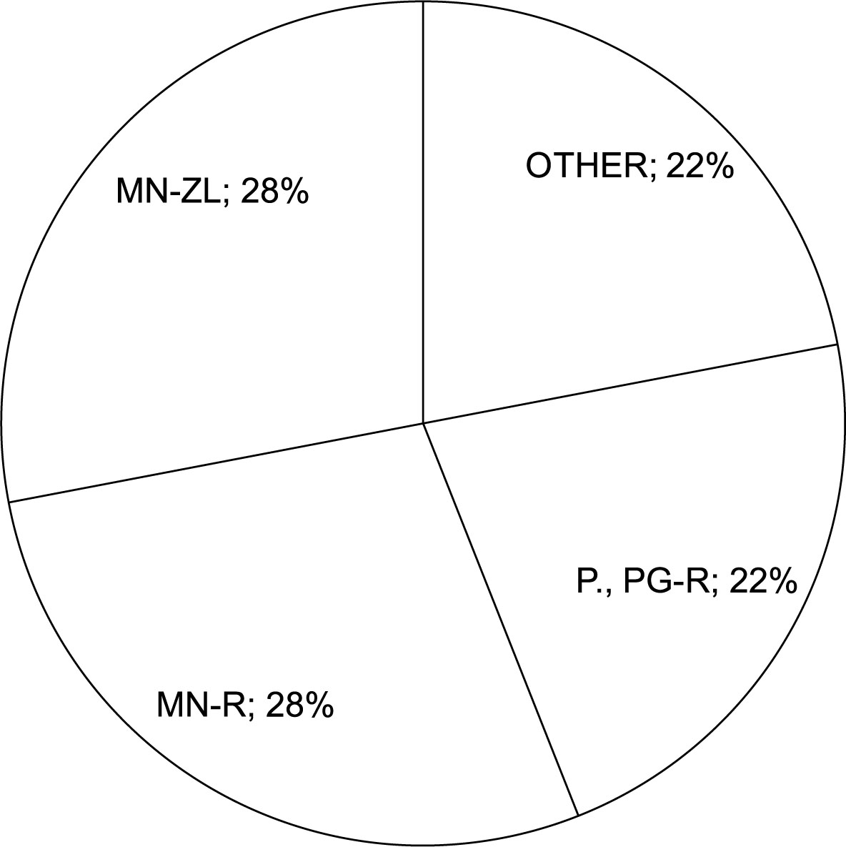
Fig. 3
Share of incompatibilities of land use allocations occurring on the border of the commune of Oleśnica – 2016.
Source: own study based on field inventory.