
Quantum key distribution (QKD) [1,2], whose security relies on the fundamental laws of quantum mechanics, is one of the most successful directions in practice in quantum information processing. Since Bennett and Brassard proposed the first standard one-way QKD protocol, namely the BB84 [1], for nearly four decades of efforts, the security proof problem of these BB84-type QKD protocols have been solved in ideal-devices settings [3–6], and the communication distance has been extended from the early 32cm [7] to 1200km satellite-to-ground [8]. In practice, the imperfect factors of QKD devices, such as imperfect single-photon sources, channel decay, and imperfect photon detectors, are vulnerable to powerful eavesdroppers, thus reducing the key performances and even compromising the security of QKD. Recently, the decoy technique [9,10] and the measurement-device-independent (MDI) proposal [11] not only close nearly all (except the characteristic of the sources) of the main current loopholes in real-life QKD devices but also significantly improve the key performance with imperfect single-photon sources. Later, MDI-QKD protocols with imperfect sources were presented, making QKD more robust in real-world applications [12,13]. However, most one-way QKD protocols are nondeterministic (in the post-processing, bases reconciliation is needed, and nearly half of the effective signal sources are sifted off to obtain raw key bits, which reduces the key rate by nearly half). Another relatively new proposal, deterministic QKD (DQKD), was proposed to amend the nondeterministic factor of one-way QKD. The two classical deterministic protocols are the Ping-Pong (PP) protocol and the LM05 protocol [14,15]. The distinct feature of the DQKD is the two-way (forward and backward) quantum channel, usually called TWQKD. The security proof is more complex as Eve can invade it in both the quantum forward channel (QFC) and the quantum backward channel (QBC). Over the past two decades, through hard work, the security of TWQKD has been proven under ideal-device settings [16–19]. It demonstrated that the performance of TWQKD can even surpass that of one-way QKD within a specific distance range, showing great potential to achieve good performance [20]. However, due to its two-way nature, TWQKD is more vulnerable when considering the loopholes of imperfect measurement devices. Eve can use it to steal partial or even complete key information [21], and the communication distance limit is relatively shorter than that of one-way QKD. Remarkably, Lu et al. take the first step to prove that DQKD is MDI secure in the QBC, while the photon detector at Alice’s side for check mode (to ensure security, check the fidelity of the QFC) is assumed to be perfect [22]. In this paper, we propose a DQKD protocol to double the limit transmission distance under the assumption that all measurement detectors, the relay, is untrusted (controlled by Eve). Later, we refer to it as the untrusted relay DQKD (UR-DQKD). The main work of this paper is to derive the performance formula for the UR-DQKD based on the current technology of QKD devices with finite sources.
The rest of this paper is arranged as follows. Details of the UR-DQKD protocol are presented in Section 2, whose key performance formula and simulation results are given in Section 3. Finally, a discussion and conclusion are made in Section 4.
As in Figure 1, without loss of generality, Bob and Alice run the protocol according to the following steps.
Preparation. First, Bob sends a communication request to Alice through an authenticated classical channel. Then, according to a random bit string with length N, denoted as b = b1b2 … bN with bi ∈ {0, 1} and i ∈ {1, 2, …, N}, Bob prepares and sends N qubits, written as a density matrix
{\rho _B} = \otimes _{i = 1}^N\rho _B^i \rho _B^i = \sum {{1 \over 4}} \left| {{\varphi ^i}} \right\rangle \left\langle {{\varphi ^i}} \right|,\left| {{\varphi ^i}} \right\rangle | \pm \rangle = {1 \over {\sqrt 2 }}|0\rangle \pm |1\rangle {\rm{qubit}}\rho _B^i Encoding mode. In the EM, Alice randomly (with equal probability) performs with two operators, I and iϒ, on the k-th qubit |φk〉 to encode bits ak. Where ak is part of a, and it will be used as the raw key bits. The unitary operator I = |0〉 〈0| + |1〉 〈1| encodes bit ak = 0 and iϒ = |0〉 〈1| – |1〉 〈0| encodes bit ak = 1. iϒ flips on all four prepared states as follows: iϒ|0〉 = –|1〉, iϒ|1〉 = |0〉, iϒ|+〉 = |–〉, iϒ|–〉 = –|+〉. After passing through the EM, all encoded qubits are sent to t+he UR.
Control mode. In the control mode (CM), according to the rest part of a, denoted as aj, j ∈ [1, N] and j ≠ k. Alice randomly (with equal probability) performs the Pauli Z operator (aj = 0) or the Pauli X operator (aj = 1) on the j-th qubit |φj〉 and then sends them to the UR.
Here, we emphasize that instead of measuring all the qubits from the CM and the EM by legitimate parties, Bob delegates the decoding measurement process to Eve and informs Eve the basis of |φi〉 through an authenticated classic channel. Eve measures each of Alice’s qubits via Bob’s basis in the UR, and then reports all of the measurement results (N bits), denoted as Ei, to Bob. Without noise, in the EM, Eve’s measurement outcomes are Ek : ak ⊕ bk, while in the CM, Eve’s outcomes are more complex, i.e., Ej = bj if the basis used by Alice matches the basis chosen by Bob, otherwise, Ej are randomly to be 0 or 1.
Security Check. Alice announces the serial number j of each |φj〉 and the corresponding control operator that is used in the CM. According to Alice’s announcement, Bob computes the quantum bit error rate (QBER) of aj, denoted as QCM. If QCM exceeds the security threshold, they regard Eve as having seriously invaded the quantum channel and abort the rest of the bits.
Key distillation. If QCM is acceptable, Alice randomly announces part of the ak to compute the QBER of ak, denoted as QEM. If QEM is acceptable (note, in the asymptotic case QEM = QCM), Alice and Bob perform the error-correction (EC) and the privacy amplification (PA) to distillate the final secure key bits.
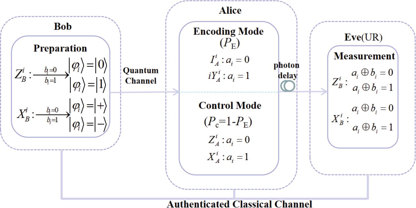
Schematic illustration of the UR-DQKD Classic.
Here, a photon delay with a small time slot may be needed in Alice’s module, as Bob only tells Eve the basis of
Here, we first emphasize and list the assumptions on which the security of this protocol is based.
First, the sources are security, i.e., the preparation basis of |φi〉 is not leaked to Eve before step 3, or in other words, the bit string b is unknown to Eve before step 3. Pre-shared entanglement between |φi〉 and Eve’s ancilla |ε〉E is also excluded.
Second, Alice’s bit string a is not leaked to Eve. Alice has free will to choose the encoding and the control operators randomly.
Third, Eve can access quantum memory devices that have for arbitrary long coherence time.
Based on the above assumptions, we can infer that the security basis of this protocol is founded on two key points. First, Eve cannot distinguish between the qubits that pass through the EM and the ones that pass through the CM until Alice’s announcements in step 4. Second, the density matrix of
Eve cannot get any information about the encoding bits ak from the measurement results Ek : ak ⊕ bk.
In the view of Eve, this protocol is equivalent to the one in which Alice randomly uses four operations {I, iY, Z, X} for encoding. Thus, due to the CM, Eve will inevitably introduce QBER if she tries to get the information of ak via attacks.
We first consider the ideas of the so-called zero-error attacks [24,25]. Suppose that, in the i-th round, Eve emits a fake state
Now we consider the security bound for this protocol under the general collective attacks [26]. Eve performs the attacks
It reveals that the quantum channel noise in this protocol constrains Eve’s ability to steal the maximum amount of information.
Here we argue that, in this protocol, Eve can not obtain more information by performing the general coherent attack mentioned in the LM05 protocol [15] than the one via the above general collective attack. In the coherent attack, in each round, Eve performs the first unitary attack
In this section, we derive the performance formula for this protocol, close to the real-world QKD system. We first present the reasonable models of the devices for this protocol, based on current technology.
We assume that Bob uses single photons as the source (SPS). In each round, Bob successfully emits a singlephoton state to the quantum channel with probability P1 (efficiency of single-photon state collection) or a vacuum state due to random losses with the probability P0, P1 + P0 = 1. Note that high-performance single-photon sources (SPS) have made significant progress in recent QKD experiments and P1 can be over 99% in practice [27]. Here we set P1 = 90%.
The quantum channel (optical fiber) transmittance tAB can be expressed as
We consider a threshold photon detector in the UR that cannot resolve the photon number of each photon pulse, but can only distinguish a vacuum pulse from a non-vacuum pulse.
Then, the total efficiency of the QKD system is η = tABηAB, where ηAB = tAtBηE denotes the total transmittance of the devices in Alice and Bob’s sides (tAtB) and the UR (ηE). Here, the efficiency of the photon delay on Alice’s side, which can be nearly unity with today’s technology, is merged into the UR.
From the above models, the performance formula for this protocol can be written as
Details of each term in Equation (2) are listed below.
The factor PEM is the probability of implementing the EM, and g is the total gain in the UR from Bob’s SPS.
ϒ1 is defined as the yield of a single-photon pulse, i.e., the condition probability of a detection event in the UR given that Bob sends out a single-photon pulse. Note that ϒ0 (typically 10−5 ~ 10 −6) is the background detection rate that is independent of the SPS detection.
e1 and eg are, respectively, the error rate of single-photon pulses and the overall QBER. fEC ≥ 1 is the directional error correction efficiency.
Usually, g and eg can be obtained directly from experiments, while the parameters ϒ1 and e1 must be estimated tightly. Here, we give the theoretically expected bound of each term in Equation (2) to get the bound of Kfinite.
The total gain g is given by
The total QBER is given by
Based on the assumption presented in [28], in the finite sources scenario, the lower bound of ϒ1 in this protocol can be written as
The upper bound of e1 is given by
According to the law of large numbers and the finite sources theorem [29–31], δϒ1 and δe are, respectively, given by
Note, ϒ1 should be tightly estimated over all N pulses, while δe should be tightly estimated only over the pulses from the EM, and this protocol has four outcomes of the positive operator-valued measurement, POVM, in the UR). Then, with the above Equations (3)–(8), we can calculate the lower bound of Kfinite. Simulation results of Equation (2) are presented in Figure 2 with the parameters of today’s QKD technology, as listed in Table 1.
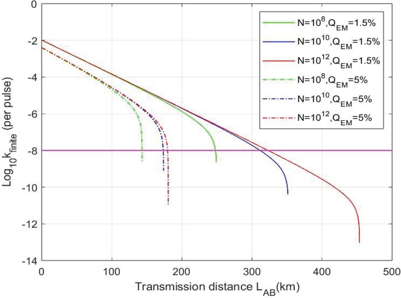
As a function of the transmission distance LAB between Alice and Bob. We simulate the lower bounds of the finite-key-rate Kfinite in three cases: (N =108) green-solid-line, (N =1010) blue-solid-line, and (N = 1012) red-solid-line, QEM = 1.5%, ηE = 14.5%; (N = 108) green-dash-dotted-line, (N = 1010) blue-dash-dotted-line, and (N = 1012) red-dash-dotted-line, QEM = 5%, ηE = 14.5%.
Experimental parameters of today’s QKD technology.
| β(dB/km) | QEM | ϒ0 | ηE | fEC | εPE |
|---|---|---|---|---|---|
| 0.2 | 1.5%∽5% | 8 × 10⁻⁸ | 14.5% ∽ 45% | 1.15 | 10−8 |
Figure 2 shows that: the finite lengths of sources have significant effects on the limit transmission distance; with QEM = 1.5%, N ≥ 108, cut off those key rates below 10−8, the performance is over 248km∽10−8 bits/pulse, and the limit transmission distance can be extended over 320 km with N ≥ 1012; even with QEM = 5%, much higher than the current value in practice, the performance is over 143km∽10−8 bits/pulse, and the limit transmission distance can be extended over 180 km with N ≥ 1012.
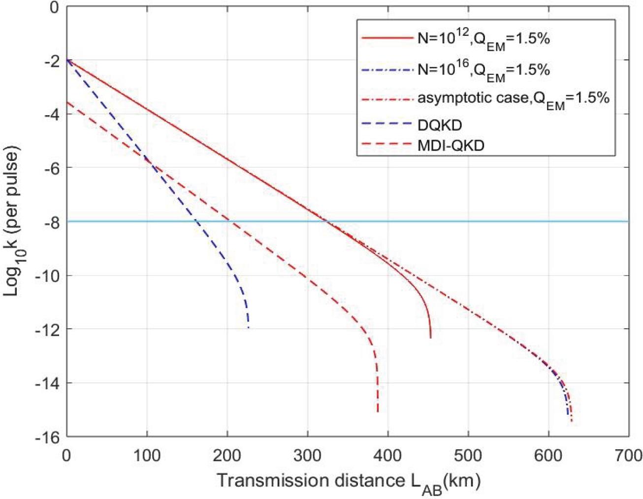
Figure 3 shows that: the UR-DQKD doubles the performance of the current DQKD, and the effect of the finite lengths of sources is negligible when N is large enough, i.e., N ≥ 1016; brief comparison with the performance of the MDI-QKD, i.e., the dashed line in Figure 3 in Ref. [32], the key rate and the limit transmission distance of this protocol perform better than that of the MDI-QKD. All critical parameters for comparison are the same as those in Table 1 (QEM = 1.5%, ϒ0 = 8 × 10⁻⁸, ηE = 14.5%, fEC = 1.15, and β = 0.2) except for the sources: infinite decoy states of coherent pulses in the MDI-QKD, finite SPS based on the recent experiment progress in this protocol. Theoretically speaking, for the MDI-QKD with infinite decoy states, besides the signal coherent pulses with intensity μAlice = μBob = μ, Alice and Bob send infinite faint coherent pulses with intensities vi(vi ∈ {v1, ν2, …, vm}, m → ∞, and vi < μ) to the UR to tightly estimate the gain Y11 and the error rate e11 of the key rate equation (B31) in Ref. [32], which makes the key rate of the MDI-QKD with infinite coherent pulses asymptotic to that of the MDI-QKD with infinite single photons. Note that the optimal μ, approximately 0.2∽0.6, slightly varies with the transmission distance LAB and is numerically optimized in Figure 3. Therefore, under the above conditions, it is justified to make a performance comparison between the infinite decoy states MDI-QKD and this UR-DQKD with finite SPS.
In this work, we propose a UR-DQKD protocol. The main work of this paper focuses on deriving the lower bound of the performance formula for it with a practical model based on today’s technology. Moreover, with the current parameters, the simulation results show that this protocol can achieve good performance. It nearly doubles the performance of the current DQKD employing a trusted relay [15] and outperforms the MDI-QKD within a considerable distance (320km). It is foreseeable that the performance will be over 470km∽10−8 bits/pulse if the critical parameters of the QKD system are set to the optimal values of today’s technology, i.e., use ultralow-loss fiber (β = 0.17) and high-efficiency detector (ηE ≥ 45%) [33], thus expected to be comparable with the performance of the PM-QKD [32]. We also note the recent progress in the experimental demonstration of quantum secure direct communication (QSDC) with single-photons and entanglement-pairs, which also indicates the potential of achieving high-performance MDI-DQKD with current devices (over 200km with relatively high secure key rates) [34]. In conclusion, this protocol is feasible with today’s technology, allowing high-performance, secure networks with a relay controlled by an untrusted third party.