
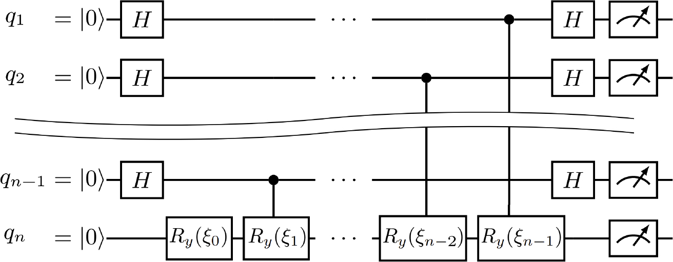
Figure 1.
Shallow circuit for quantum fingerprinting or quantum hashing algorithm.
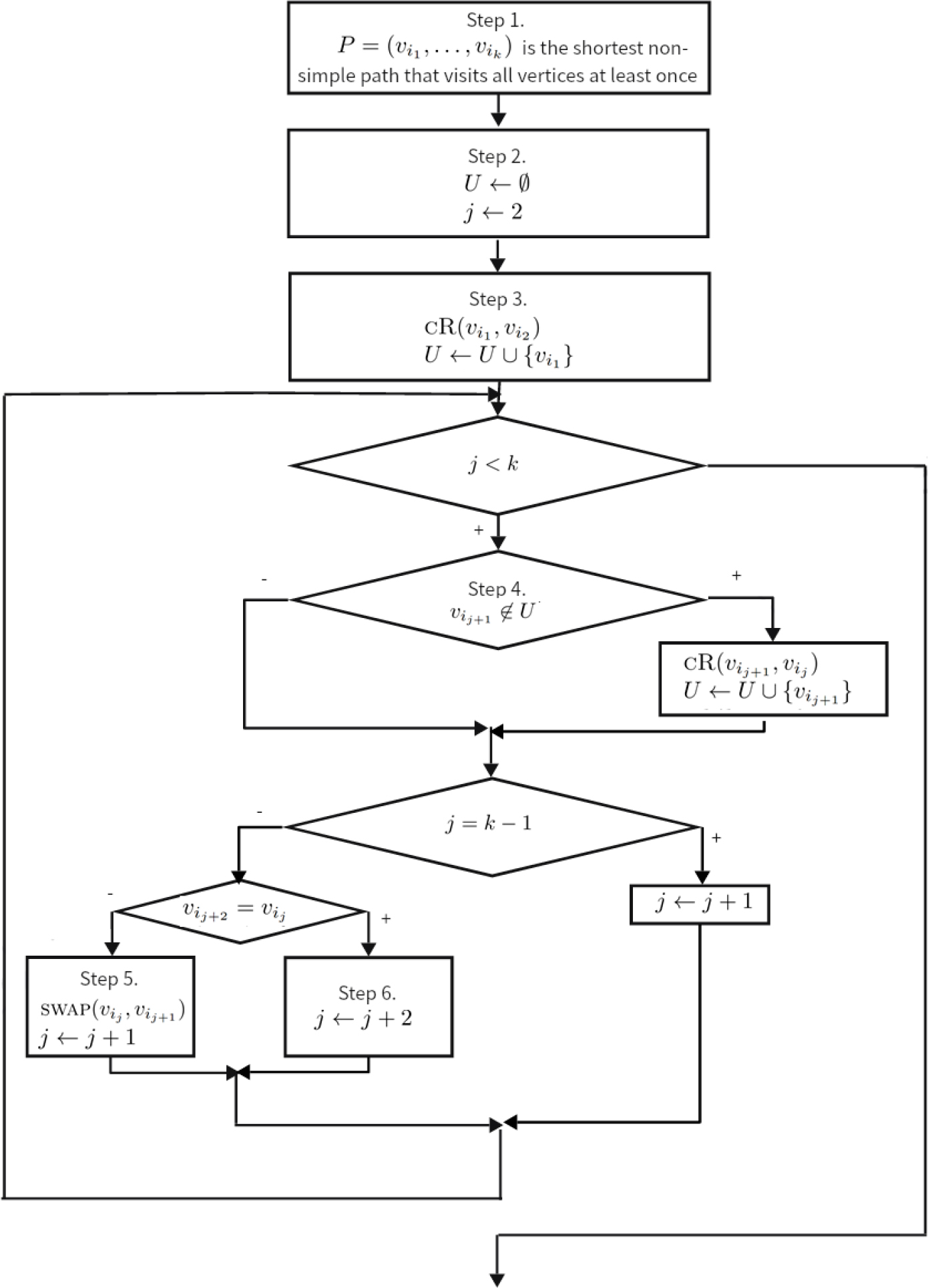
Figure 2.
The flowchart for algorithm constructing a circuit for quantum hashing.

Figure 3.
Representation of CRy gate using only basic gates
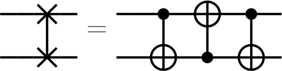
Figure 4.
Representation of SWAP gate using only basic gates

Figure 5.
Representation of a pair CRy and SWAP gates using only basic gates
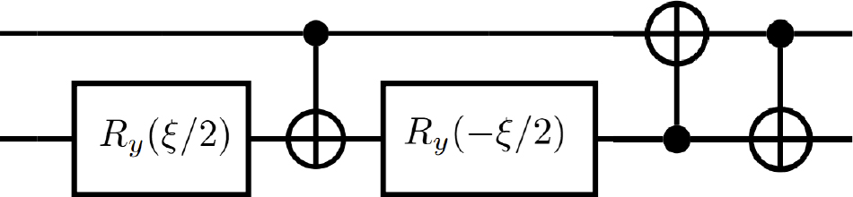
Figure 6.
Reduced representation of a pair CRy and SWAP gates using only basic gates

Figure 7.
The graph for the 5-qubit LNN architecture. The path that visits all vertices at least once is green.
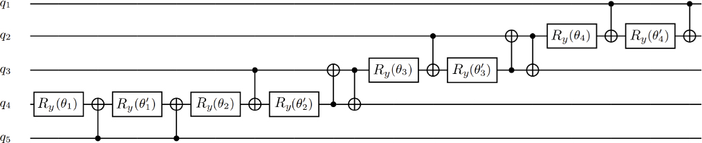
Figure 8.
A quantum circuit for the Quantum hashing (quantum fingerprinting) algorithm for 5 qubits LNN architecture device.
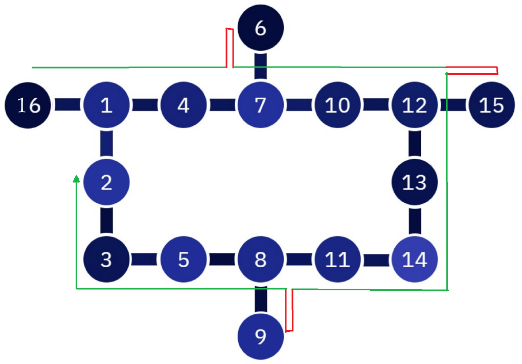
Figure 9.
The graph for 16-qubit “sun” architecture. The path that visits all vertices at least once is green. Red parts are such that vij = vij+2.
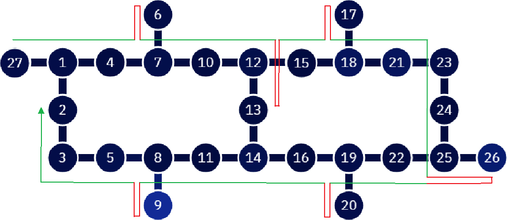
Figure 10.
The graph for 27-qubit “two joint suns” architecture. The path that visits all vertices at least once is green. Red parts are such that vij = vij+2.
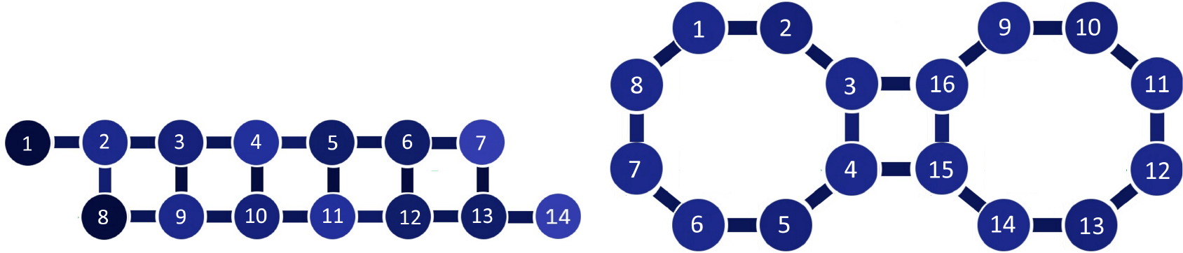
Figure 11.
Connectivity graphs of IBMQ Melbourne, Regetti Aspen-4, and 5 × 5-grid.
Table 1.
The CNOT cost for the LNN architecture. The CNOT cost of circuits produced by algorithms from [79] and this paper is 3n – 5
| The number of qubits n | [79] and this paper | Qiskit transpiler |
|---|---|---|
| 5 | 10 | 14 |
| 10 | 25 | 39 |
Table 2.
The CNOT cost for “sun” and “two joint suns” architectures
| Connectivity graph’s type | [23] and this paper | Qiskit transpiler |
|---|---|---|
| 16-qubit “sun” architecture | 40 | 57 |
| 27-qubit “two joint suns” architecture | 69 | 115 |
Table 3.
The CNOT cost for IBMQ Melbourne, Regetti Aspen-4, and 5 × 5-grid
| Connectivity graph’s type | This paper | Qiskit transpiler |
|---|---|---|
| 14-qubit IBMQ Melbourne | 36 | 44 |
| 16-qubit Regetti Aspen-4 | 43 | 66 |
| 25-qubit 5 × 5-grid | 70 | 84 |
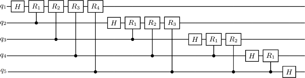
Figure 12.
A quantum circuit for the Quantum Fourier Transform algorithm for fully connected 5 qubits.

Figure 13.
Representation of CRd gate using only basic gates.

Figure 14.
Reduced representation of a pair Rd and SWAP gates using only basic gates.
Table 4.
Table 5.
The CNOT cost of quantum circuit for the QFT algorithm for “sun” and “two joint suns” architectures
| Connectivity graph’s type | This paper | [23] | Qiskit transpiler |
|---|---|---|---|
| 16-qubit “sun” architecture | 342 | 324 | 549 |
| 27-qubit “two joint suns” architecture | 1009 | 957 | 1839 |
Table 6.
The CNOT cost of quantum circuit for the QFT algorithm for IBMQ Melbourne, Regetti Aspen-4, and 5 × 5-grid
| Connectivity graph’s type | This paper | Qiskit transpiler |
|---|---|---|
| 14-qubit IBMQ Melbourne | 269 | 335 |
| 16-qubit Regetti Aspen-4 | 359 | 585 |
| 25-qubit 5 × 5-grid | 899 | 1158 |
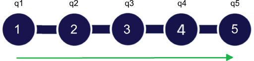
Figure A1.
The graph for the 5-qubit LNN architecture. The path that visits all vertices at least once is green. q1, …, q5 are assigned logical qubits for the vertices.

Figure A2.
The circuit for the first cascade.
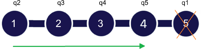
Figure A3.
The graph for the 5-qubit LNN architecture. The second cascade excludes the vertex that corresponds to 1-st logical qubit. The path that visits all vertices at least once is green.
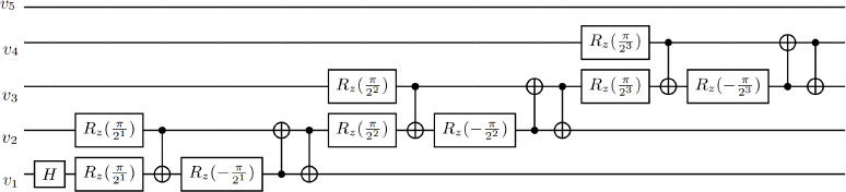
Figure A4.
The circuit for the second cascade.
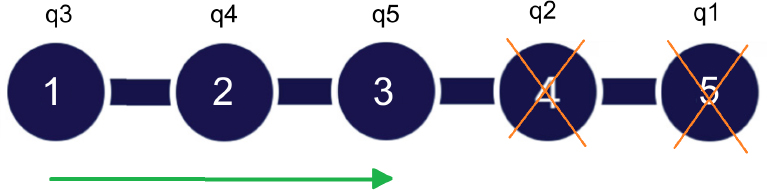
Figure A5.
The graph for the 5-qubit LNN architecture. The 3rd cascade excludes the vertices that correspond to 1st and 2nd logical qubits. The path that visits all vertices at least once is green.
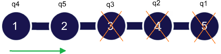
Figure A6.
The graph for the 5-qubit LNN architecture. The 4th cascade excludes the vertices that correspond to 1st, 2nd, and 3rd logical qubits. The path that visits all vertices at least once is green.

Figure A7.
The circuit for the 3rd, 4th, and 5th cascades.
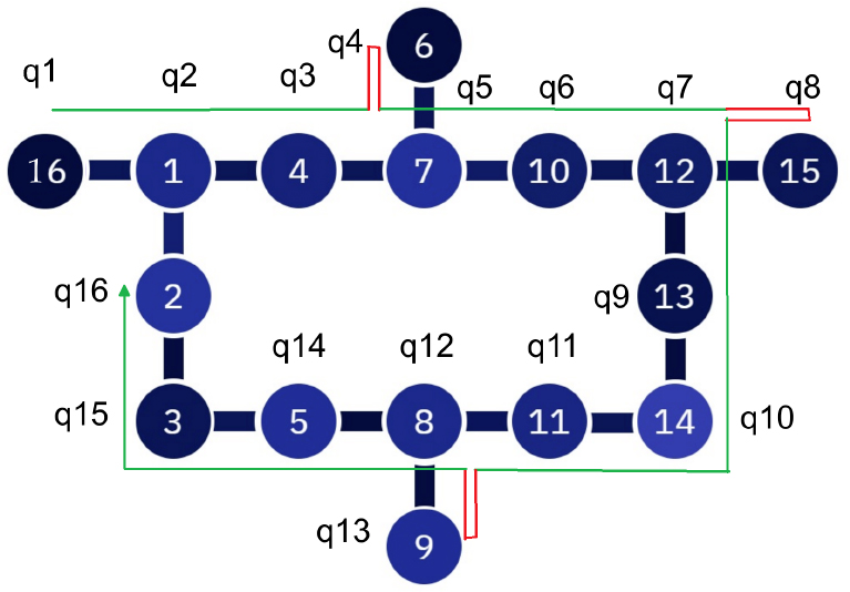
Figure A8.
The graph for the 16-qubit “sun” architecture. The path that visits all vertices at least once is green. Red parts are such that vij = vij+2. The labels q1, …, q16 are names of assigned logical qubits for the vertices.
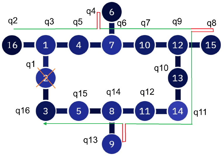
Figure A9.
The graph for the 16-qubit “sun” architecture. The second cascade excludes the vertex that corresponds to the 1-st logical qubit. The path that visits all vertices at least once is green. Red parts are such that vij = vij+2.
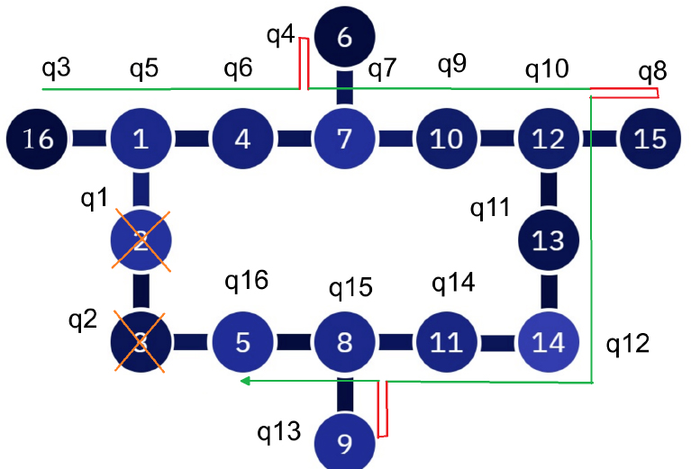
Figure A10.
The graph for the 16-qubit “sun” architecture. The 3rd cascade excludes the vertex that corresponds to the logical qubits with indices from the {1, 2} set.
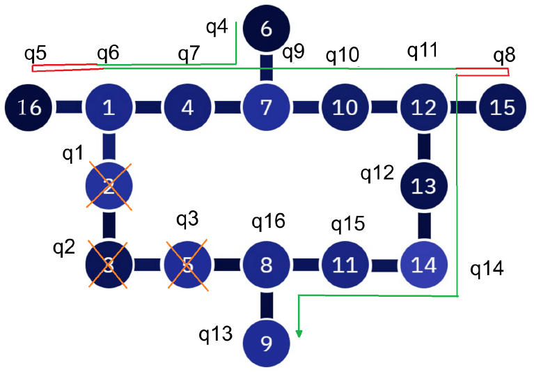
Figure A11.
The graph for the 16-qubit “sun” architecture. The 4th cascade excludes the vertex that corresponds to the logical qubits with indices from the {1, 2, 3} set.
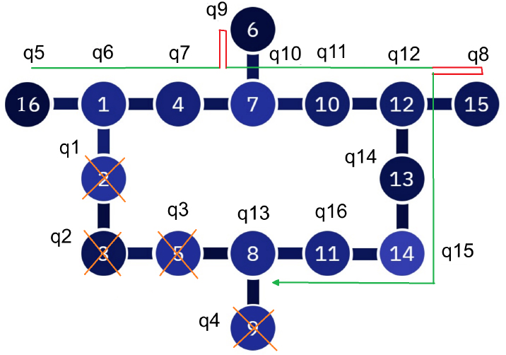
Figure A12.
The graph for the 16-qubit “sun” architecture. The 5th cascade that excludes the vertex that corresponds to the logical qubits with indices from the {1, …, 4} set.
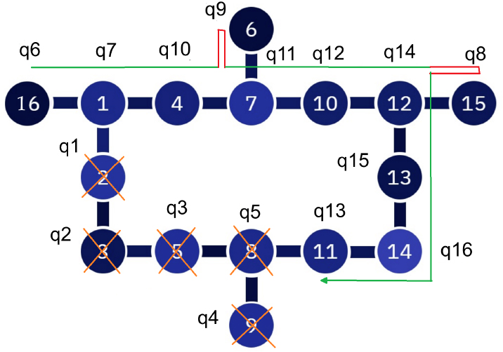
Figure A13.
The graph for the 16-qubit “sun” architecture. The 6th cascade that excludes the vertex that corresponds to the logical qubits with indices from the {1, …, 5} set.
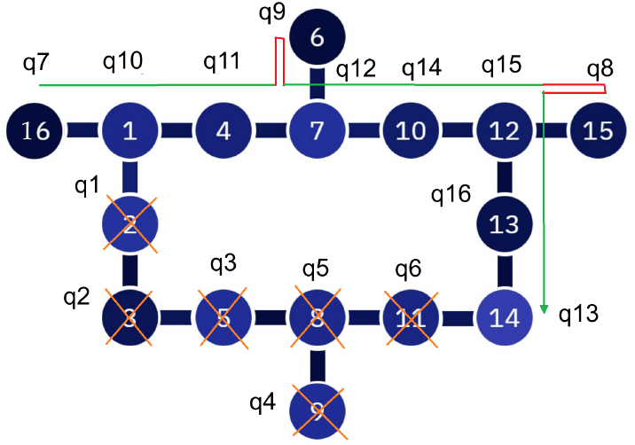
Figure A14.
The graph for the 16-qubit “sun” architecture. The 7th cascade that excludes the vertex that corresponds to the logical qubits with indices from the {1, …, 6} set.
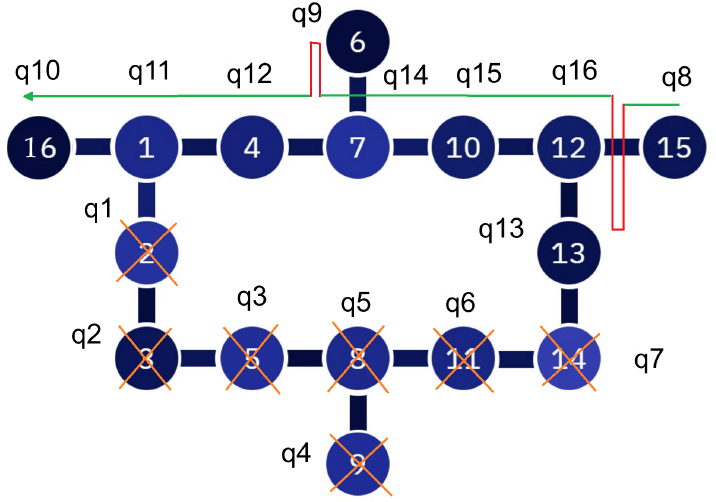
Figure A15.
The graph for the 16-qubit “sun” architecture. The 8th cascade that excludes the vertex that corresponds to the logical qubits with indices from the {1, …, 7} set.
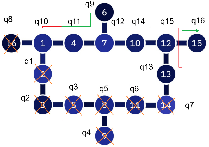
Figure A16.
The graph for the 16-qubit “sun” architecture. The 9th cascade that excludes the vertex that corresponds to the logical qubits with indices from the {1, …, 8} set.
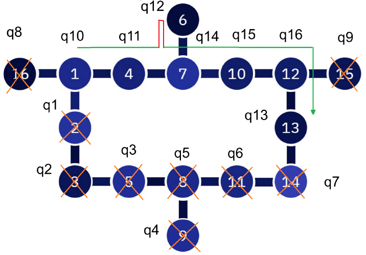
Figure A17.
The graph for the 16-qubit “sun” architecture. The 10th cascade that excludes the vertex that corresponds to the logical qubits with indices from the {1, …, 9} set.
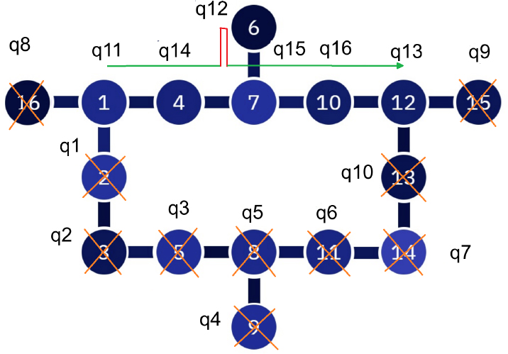
Figure A18.
The graph for the 16-qubit “sun” architecture. The 11th cascade excludes the vertex that corresponds to the logical qubits with indices from the {1, …, 10} set.
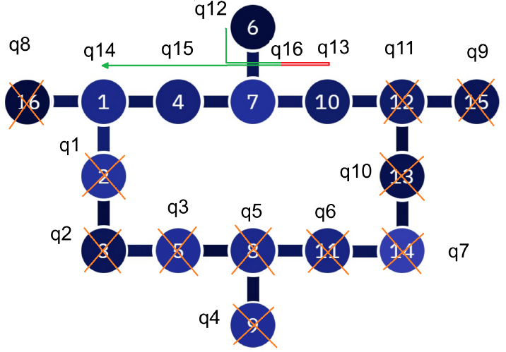
Figure A19.
The graph for the 16-qubit “sun” architecture. The 12th cascade excludes the vertex that corresponds to the logical qubits with indices from the {1, …, 11} set.
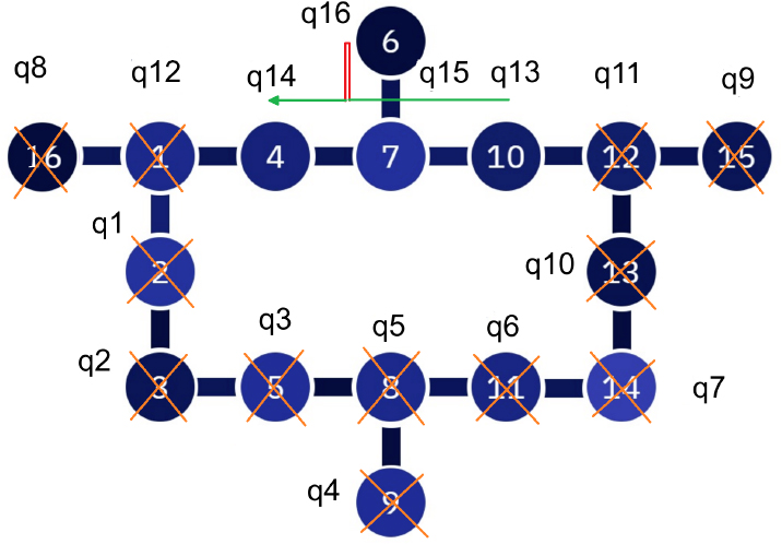
Figure A20.
The graph for the 16-qubit “sun” architecture. The 13th cascade excludes the vertex that corresponds to the logical qubits with indices from the {1, …, 12} set.
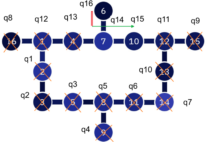
Figure A21.
The graph for the 16-qubit “sun” architecture. The 14th cascade excludes the vertex that corresponds to the logical qubits with indices from the {1, …, 13} set.
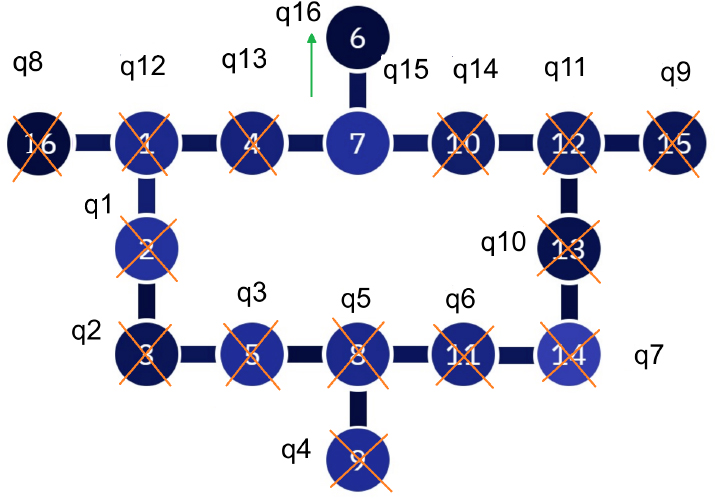
Figure A22.
The graph for the 16-qubit “sun” architecture. The 15th cascade excludes the vertex that corresponds to the logical qubits with indices from the {1, …, 14} set.
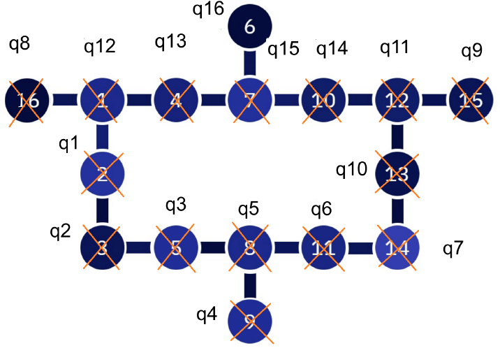
Figure A23.
The graph for the 16-qubit “sun” architecture. The 16th cascade excludes the vertex that corresponds to the logical qubits with indices from the {1, …, 15} set.