
The quantum Fourier transform (QFT) [1] is a well-known computational technique used in many quantum algorithms. The technique is used in quantum addition [2], quantum phase estimation (QPE) [1], quantum amplitude estimation (QAE) [3], the algorithm for solving linear systems of equations [4], Shor’s factoring algorithm [5], 1D wave equation [6], Quantum walks [7–9] with applications to quantum backtracking [10,11] and others.
In this paper, we are interested in the implementation of this technique on quantum devices as a quantum circuit with basic gates. There are different ways to optimize the circuits, such as invoking it in a parallel way [12] or approximate QFT [13]. We are focusing on the minimization of two-qubit quantum gates in such a circuit because they are the most “expensive” to implement. Many types of quantum computers (e.g., quantum devices based on superconductors) do not allow us to apply two-qubit gates to an arbitrary pair of qubits but have a graph that represents such a restriction. Vertices of the graph correspond to qubits, and two-qubit gates can be applied only to qubits corresponding to vertices connected by an edge. We say that such a graph represents the qubit topology for a device. In this paper, we focus on the number of CNOT gates in a quantum circuit for the QFT algorithm with respect to such a graph. Let a CNOT cost of a circuit be the number of CNOT gates in the circuit. The CNOT cost for a linear nearest-neighbor (LNN) architecture (where the graph is just a chain) was explored by Park and Ahn in [14]. They presenteda circuit that has n2 + n – 4 CNOT cost, where n is the number of qubits. It improved the previous results of [15–22]. At the same time, as the authors mentioned, their technique cannot be generalized to more complex graphs. Khadieva in [23] suggested a quantum circuit for a more complex architecture that is a cycle with tails (like a “sun” or “two joint suns”). At the same time, the CNOT cost of this circuit is 1.5n2.
Here, we present a general method that allows us to develop a quantum circuit of the QFT algorithm for an arbitrary connected graph that represents a qubit connectivity graph. Our solution is based on a solution for the Travelling salesman problem (TSP) for a modification of the original graph. Here we present a method and an algorithm for constructing a circuit with O(n22n) time complexity, where n is the number of vertices of the original graph and the approximate solution with polynomial time complexity O(n6) and the differential approximation ratio
The constructed circuit has the CNOT cost from n2 – n – 4 to 3n2 – 3n – 10 depending on the complexity of the graph. If the graph has a Hamiltonian path, then it has the minimum possible CNOT cost at most 1.5n2 – 1.5n – 1. In addition, we compare our results with circuits for specific graphs. In the case of LNN, the CNOT cost is 1.5n2 – 1.5n – 1, that is, 1.5 times larger than the result of [14]. The circuits built by our approach are larger by n CNOT gates than the circuit of [23] with the CNOT cost 1.5n2 – 2.5n – 1. For more complex graphs such as 16-qubit and 27-qubit Eagle r3 architectures of IBMQ that is a cycle with tails (like a “sun”) or its modifications, our generic technique gives a CNOT cost a bit larger than the circuit [23] that was especially constructed for these architectures. Our circuits have CNOT cost 342 for the 16-qubit architecture and 1009 for the 27-qubit one; and [23] has CNOT cost 324 and 957, respectively. The difference is about 5%.
Another technique discussed in this paper is quantum fingerprinting, or quantum hashing. This technique is well known, and it allows us to compute a short hash or fingerprint that identifies an original large data with high probability. The nature of the technique and its implementation is similar to the QFT algorithm [23,24].
The probabilistic (randomized) technique was developed by Frievalds [25]. Then, Ambainis and Frievalds [26] developed its quantum counterpart for automata that was improved by Ambainis and Nahimovs in [27,28]. Later, Buhrman et al. in [29] provided an explicit definition of the quantum fingerprinting technique to construct an efficient quantum communication protocol for equality testing. The technique was applied for branching programs by Ablayev, Gainutdinova, Vasiliev, and co-authors [30–34]. Later, they developed the concept of cryptographic quantum hashing [35–46]. Then, different versions of hashing functions were applied by Ablayev, Vasiliev, Ziiatdinov, Zinnatullin, and other researchers [24, 47–50]. The technique was also extended for qudits [51]. This approach was widely used in different areas like stream processing algorithms [52,53], query model algorithms [54,55], online algorithms [56–62], branching programs [63–65], developing quantum devices [66], automata (discussed earlier, [67–71]), and others.
Turaykhanov, Akat’ev, and co-authors implemented the technique in a real quantum device based on photons [72,73]. The alternative implementation for photon-based real quantum devices was developed by Plachta et al. [74] and Zhao et al. [75]. At the same time, the algorithm was embedded in this device. When we discuss the implementation of the algorithm for “universal” quantum devices such as IBMQ quantum computers or similar, it is important to minimize the number of quantum gates with respect to the architecture restrictions of a quantum device, as we discussed for QFT above. The basic implementation part of quantum hashing circuits is a uniformly controlled rotation operator. The CNOT cost of this operator with respect to the qubit connectivity graph was previously discussed in [76,77] for the linear nearest-neighbor (LNN) architecture and in [78] for more complex graphs. At the same time, the presented approaches have issues with the rotation angle precision, which cannot be too small. This issue is discussed in [79,80].
Kālis in his master’s thesis [81] suggested a shallow circuit for quantum fingerprinting for 3 qubits. Later, the approach was developed in detail and presented in a general way for quantum hashing by Ziatdinov, Khadieva, and Yakaryilmaz [82,83]. The approach allows us to reduce the number of CNOT gates exponentially in computational experiments. At the same time, the theoretical exponential superiority of the shallow circuit is not shown [82,83]. By the way, the method is very perspective for current and near-future quantum devices that definitely cannot support a huge number of CNOT gates. The efficient implementation of the shallow circuit for an automaton that recognizes the MODp = {ak : k mod p = 0} language based on the quantum hashing algorithm was proposed by Khadieva, Salehi, and Yakaryilmaz [79] for devices based on the LNN architecture. Later, a similar technique was applied by Khadieva [23] for a more complex architecture that is a cycle with tails (like a “sun” and “two joint suns”) represented by 16-qubit and 27-qubit Eagle r3 IBMQ architectures. Vasiliev [84] discussed a similar method, but for Rz gates instead of Ry gates.
In this paper, we present a general method that allows us to develop a quantum circuit of the quantum hashing algorithm for an arbitrary qubit connectivity graph. It uses the same tools and approaches as the algorithm for constructing the circuit of QFT. Note that the shallow circuit for quantum fingerprinting and the circuit for QFT have similar structures as was discussed by Khadieva [23]. That is why we consider these two topics together and use common methods for both algorithms.
The CNOT cost of the constructed circuit is from 2n – 2 to 6n – 11 depending on the complexity of the graph. The presented cost value is for one implementation step of the quantum hashing algorithm. If we present the complexity of ℓ steps of the algorithm, then the constructed circuit has the CNOT cost from (2n – 4)ℓ + 2 to (6n – 13)ℓ + 2, which depends on the complexity of the graph. When we apply our approach to the LNN architecture, we obtain a circuit with the same CNOT cost as the circuit specially built for the LNN architecture [79]. If we consider 16- and 27-qubit Eagle r3 IBMQ architectures, then we have a similar situation [23].
The structure of this paper is as follows: Section 2 describes the required notations and preliminaries. Graph theory tools are presented in Section 3. Section 4 provides an algorithm for generating a quantum circuit for quantum hashing. The circuit for the quantum Fourier transform is discussed in Section 5. The final Section 6 concludes the paper and contains some open questions.
Consider an undirected unweighted graph G = (V, E), where V is the set of vertices and E is the set of undirected edges. Let n = |V| be the number of vertices, and m = |E| be the number of edges.
A non-simple path P is a sequence of vertices (vi1, …, vih) that are connected by edges, i.e., (vij, vij+1) ∈ E for all j ∈ {1, …, h – 1}. A path is called a non-simple cycle if vi1 = vih. Note that a non-simple path and a non-simple cycle can contain duplicates. Let the length of the path be the number of edges in the path, len(P) = h – 1.
A path P = (vi1, … vih) is called simple if there are no duplicates among vi1, …, vih. A simple cycle C = (vi1 … vih) is a non-simple path with only one duplicate vi1 = vih. The distance dist(v, u) is the length of the shortest path between vertices v and u.
Let N
Let us consider an undirected weighted graph S = (V′, E′), where V′ is the set of vertices, and E′ is the set of undirected weighted edges. Let w : V′ × V′ → ℝ be a weight function. We assume that w(v, u) = ∞ if (v, u) ∉ E.
For a path P = (vi1, …, vih),the length w(P) is the sum of edge weights in the path, i.e.,
Quantum circuits consist of qubits and gates. A state of a qubit is a column vector from the ℋ2 Hilbert space. It can be represented by a0|0〉 + a1|1〉, where a0, a1 are complex numbers such that |a0|2 + |a1|2 = 1, and |0〉 and |1〉 are unit vectors. Here we use the Dirac notation. A state of n qubits is represented by a column vector from the ℋ2n Hilbert space. It can be represented by
As basic gates, we consider the following ones:
Additionally, we consider five non-basic gates
The reader can find more information about quantum circuits in [15,85,86]
Let us consider an undirected unweighted connected graph G = (V, E) such that n = |V| is the number of vertices and m = |E| is the number of edges.
In this section, we consider the problem of searching for the shortest non-simple path in the graph G that visits all vertices at least once. Formally, we want to construct a non-simple path P = (vi1, …, vik) such that
the path visits all vertices, i.e., {vi1, …, vik} = V; and
the length of the path P is as small as possible.
The problem is close to the Hamiltonian path problem [87], but here we are allowed to visit a vertex several times. That is why any connected graph has the required path.
To solve this problem, we construct a new complete weighted graph S = (V′, E′) such that
The set of vertices V′ is the same as the set of vertices V.
Each pair of vertices u′, v′ ∈ V′ is connected, and the weight w(u′, v′) is the length of the shortest path between the corresponding vertices u and v from V, i.e., w(u′, v′) = dist(u, v).
We call it the “supergraph.” Let a TSP path (or a Travelling salesman problem path) P′ be the shortest simple path in S that visits all vertices from V′ exactly once [87]. In a similar way, we can define a TSP cycle C′.
For a TSP path P′ = (vi1, …, vin), let α(P′) be the path in G such that
Here Pvi1, vi2 is the shortest path in G between vi1 and vi2; the path
A TSP path for S and the shortest non-simple path in G that visits all vertices at least once has the following connection.
The shortest non-simple path P in G that visits all vertices can be obtained by a TSP path P′ for S as P = α(P′).
Let P = α(P′). Assume that there is another non-simple path
There is also a similar connection for cycles.
The shortest non-simple cycle C in G that visits all vertices can be obtained by a TSP cycle C′ for S as C = α(C′).
The proof is the same as for Lemma 1.
We can note the following property:
The length of the shortest non-simple path P that visits all vertices in G at least once is such that n – 1 ≤ len(P) ≤ 2n – 2. A similar result is for a cycle C, i.e., n ≤ len(C) ≤ 2n – 2
Let us consider a spanning tree of the graph G = (V, E). It is a tree T = (V, E′), where E′ ⊂ E. The path should visit all vertices. So, we can construct a non-simple path P that is the Euler tour [87] of the tree T. The path covers all the vertices of the graph G, but may not be the shortest. Each edge in the tour is visited at most twice (in the up- and down-direction). There are n – 1 edges in the tree. Therefore, the length of the path is at most 2n – 2. For a cycle, we have a similar situation.
Based on this connection, we can suggest an algorithm for searching the shortest non-simple path in the graph G that visits all vertices at least once.
Assume that we have a procedure that finds a TSP path for S that is TSP
Additionally, we have a procedure S
Elements of the matrix W are the lengths of the shortest paths between each pair of vertices in G, i.e., W[v, u] = dist(v, u). We can use W as a weight matrix for S. In other words, w(v′, u′) = W[v, u], where v′, u′ ∈ V′, and v and u are the corresponding vertices from V.
The matrix A represents the shortest paths between the vertices of G. The element A[v, u] is the last vertex before u in the shortest path from v to u. In other words, if t = A[v, u], then Pv, u = Pv, t ⚬ u. Based on this fact, we can present a procedure G
t ← A[v, u]
Pv, u ← (u)
while t ≠ v do
Pv, u ← (t) ⚬ Pv, u
t ← A[v, t]
end while
Pv, u ← (v) ⚬ Pv, u
return Pv, u
Let the procedure G
We can construct these two matrices using n invocations of the Breadth First Search (BFS) algorithm [87]. The total time complexity for the construction of the matrices is O(n3). The algorithm for constructing A and W is presented in Appendix D for completeness of presentation.
Due to V′= V, and the matrix W representing the weights of the supergraph’s edges, we can say that S
Finally, we can present Algorithm 2 to solve the problem.
W, A ← S
(vi1, …, vik) = P′ ← TSP
α(P′) ← G
for j ∈ {2, …, k – 1} do
α(P′) ← α(P′) ⚬ G
end for
Note that if we replace the procedure TSP
The time complexity of the presented solution for searching the shortest non-simple path, a path with a fixed starting vertex or a cycle that visits all vertices at least once in the graph G = (V, E) is O(n22n), where n = |V|.
We can solve the same problem using quantum algorithms. For TSP
The query complexity of the algorithm [90] presented by Ambainis et al. is O* (1.728n), where O* hides logfactors. The algorithm is based on the Grover search algorithm, whose time complexity is more than the query complexity for an additional log factor [94,95]. So, the time complexity is also O* (1.728n). If we want to discuss it more precisely, then we can check [90,96] which claims the query complexity O(n31.728n).
Finally, the complexity of the quantum algorithm for the problem is O* (1.728n). At the same time, for current applications, we need only a classical solution.
In the practical case, when we have more than 20–30 vertices in a graph, the exact algorithm presented before is too slow. In this section, we present a heuristic solution with polynomial-time complexity, and the outcome is close, under certain criteria, to the optimal solution.
Using a path P = (vi1, …, vih), we can construct a sequence of edges ((vi1, vi2), (vi2, vi3), …, (vih–1, vih)). We can say that these are two equivalent representations of the path. We use both in this section.
Note that the supergraph S defined in Section 3 satisfies the following conditions:
S is complete and weighted.
The weight of an edge from S is at most n because it is the distance between two vertices in the original graph. Formally, w(v′, u′) = dist(v, u) ≤ n, where v′, u′ ∈ V′, and v, u ∈ V.
S is metric. This means that the edges satisfy the triangle inequality:
w\left( {v_i^\prime ,v_j^\prime } \right) \le w\left( {v_i^\prime ,v_k^\prime } \right) + w\left( {v_k^\prime ,v_j^\prime } \right) v_i^\prime ,v_j^\prime ,v_k^\prime \in {V^\prime }
Now we present a heuristic procedure 2-O
We assume that we have two operations for modification of the list of edges that represents a cycle C:
R
eplace (C, (vij, vij+1), (u, v)) that replaces the edge (vij, vij+1) in C by the edge (u, v)R
everse (C, (vij, vij+1), (vik, vik+1)) that reverses all elements of the list between (vij, vij+1) and (vik, vik+1). Both elements (vij, vij+1) and (vik, vik+1) remain in place.
Both operations can be implemented with O(1) time complexity if C is implemented by the two-directional Linked List data structure [87].
Firstly, we initialize the cycle by ((v1, v2), …, (vn–1, vn), (vn, v1)). Then we repeatedly replace two edges of the cycle as long as this yields a shorter cycle. We check all possible pairs. The implementation is presented in Algorithm 3.
In the case of searching for a path, we have two modifications. That is, if a starting vertex vs and a finishing vertex vf are fixed, then we initialize the path by
Without loss of generality, we can assume that s < f. If the starting and finishing vertices are not fixed, then we check all possible vertices from V′ as vs and vf.
Experiments on real-world instances have shown that 2-O
C((v1, v2), …, (vn–1, vn), (vn, v1))
stopFlag ← False
while stopFlag = False do
stopFlag → True
for k ∈ {1, …, n} do
for j ∈ {k + 1,…, n} do
if w(vik, vik+1) + w(vij, vij+1) > w(vik, vij) + w(vik+1, vij+1) then
R
R
R
stopFlag ← False
break both For-loops
end if
end for
end for
end while
return C
The time complexity of 2-O
Initialization of C takes O(n) time. Since the weights of the edges are bounded above by n, the weight of any Hamiltonian cycle C is bounded above by n2. In each step of “replacing two edges,” the weight of C is reduced by at least 1, which implies that there are O(n2) steps of “replacing two edges.” In each step, there are O(n2) pairs of edges to compare, and the comparison and replacement of edges takes constant time. In summary, the total complexity is O(n4).
In the case of a path with a fixed starting vertex, we also check all finishing vertices. The number of finishing vertices is n. So, the complexity is O(n5) for searching the path.
In the case of a path, we also check all starting vertices. The number of starting vertices is n. So, the complexity is O(n6) for searching the path.
The heuristic algorithm 2-O
Let I be an input and 𝒜 be an approximation algorithm. Let lenopt (I) be the length of a path that returns an optimal solution for the given instance I. Let lenw(I) be the worst possible length that a feasible solution returns for I. Let len𝒜 (I) be the length of the approximation algorithm’s solution. Then, for an instance I
the standard approximation ratio is
{{\rm{\rho }}_{\cal A}}(I) = {{le{n_{\cal A}}(I)} \over {le{n_{opt}}(I)}} the differential approximation ratio is
{\delta _{\cal A}}(I) = {{\left| {le{n_w}(I) - le{n_{\cal A}}(I)} \right|} \over {\left| {le{n_w}(I) - le{n_{opt}}(I)} \right|}}.
Note that if the ratios are close to 1, then the algorithm has better quality.
For the heuristic algorithms for the traveling salesman problem, we have the following results.
The differential approximation ratio for the 2-O
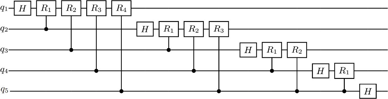
In this section, we present a method that allows us to construct a circuit for the quantum fingerprinting or quantum hashing algorithm for a connected graph G = (V, E) that is the qubit connectivity graph for a device. More information on the quantum fingerprinting (quantum hashing) algorithm can be found in Appendix B. Here we consider a shallow circuit [81,82] for n control qubits. If we do not have restrictions for applying two-qubit gates (when G is a complete graph or a “star” graph), then the circuit is such that we presented in Figure 1. Here we assume that we have qubits q1, …, qn such that q1, …, qn–1 are control ones and qn is the target one.
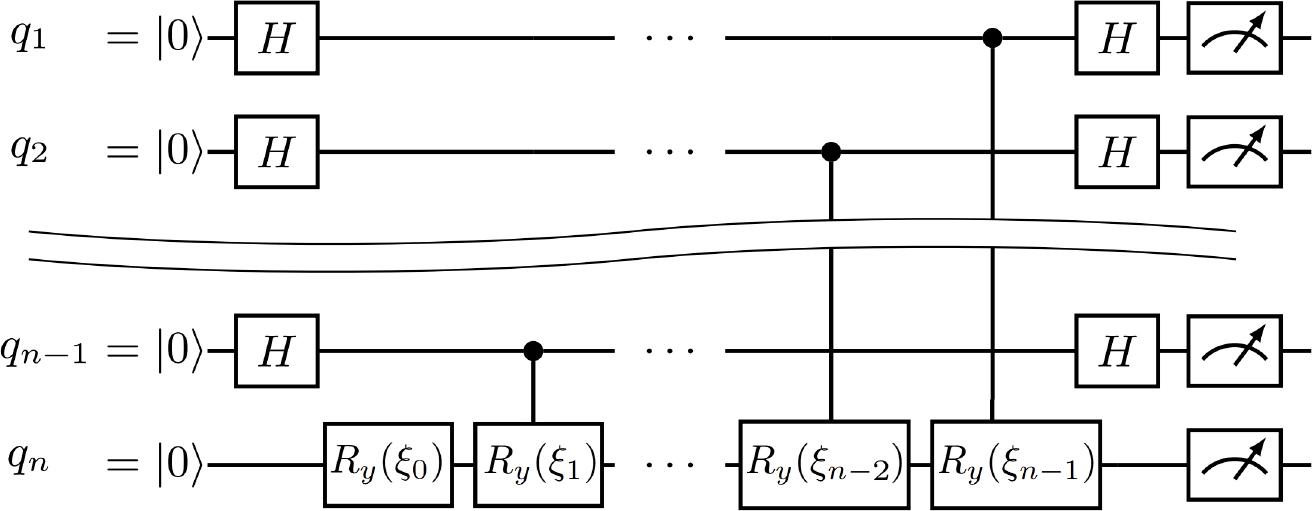
Shallow circuit for quantum fingerprinting or quantum hashing algorithm.
Let qi be the logical qubits of the original circuit; the qubits of a physical device are associated with vertices of the graph G, and we call them vi.
The algorithm for constructing a circuit is the following. We also present it in a flowchart in Figure 2.
- Step 1.
We find the shortest non-simple path in the graph G that visits all vertices at least once using the algorithm from Section 3. Assume that the path is P = (vi1, …, vik).
- Step 2.
The target qubit qn corresponds to the vertex vi2. The control qubits q1, …, qn–1 correspond to other vertices. We assume that we have a set U of control qubits that are already used. Initially, it is empty U ← ∅. Let j be the index of the element in the path P that corresponds to the target qubit. Initially, j ← 2.
- Step 3.
We apply controlled rotation with the control vi1 and the target vi2 qubits. Then, we add vi1 to the set U, i.e., U ← U ∪ {vi1}.
In the next steps the target qubit travels along the path P.
- Step 4.
If vij+1 ∉ U, then we apply a controlled rotation to the control vij+1 and the target vij qubits. After that, we add vij+1 to the set U, i.e., U ← U ∪ {vij+1}. If j = k – 1, then we terminate the algorithm. Otherwise, we go to Step 5.
- Step 5.
If vij+2 ≠ vij, then we continue; otherwise, we go to Step 6. We apply the SWAP gate to vij and vij+1. After that, we update j ← j + 1 because the value of the target qubit moves to vij+1. Then, we go to Step 4.
- Step 6.
If vij+2 = vij, then we update j ← j + 2. Note that here we stay on the same vertex of the graph G. Then, we go to Step 4.
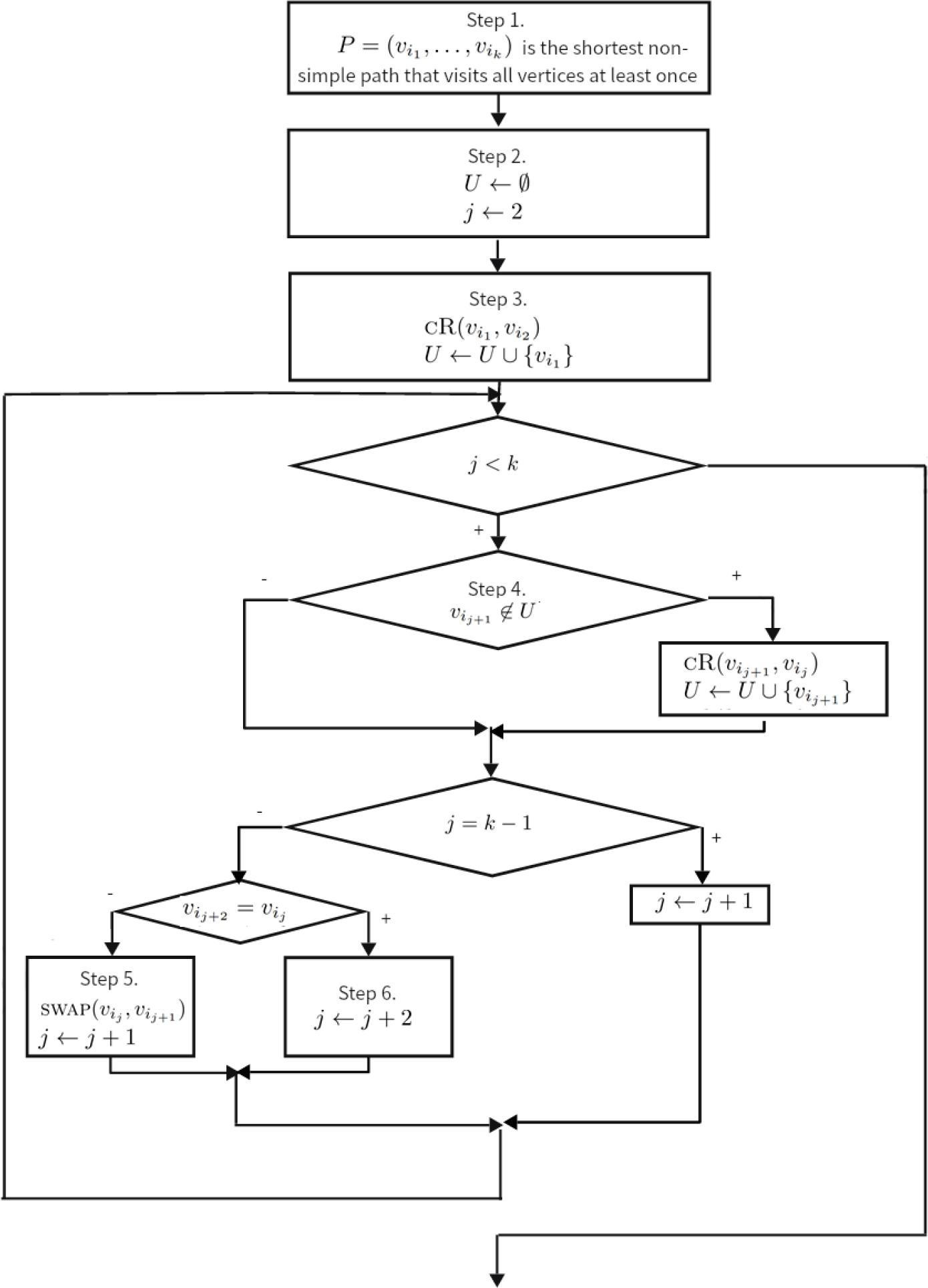
The flowchart for algorithm constructing a circuit for quantum hashing.
Let us present a procedure C
We assume that S
Let us look to the shortest path P = (vi1, …, vk) that visits all vertices at least once.
The shallow circuit (Figure 1) is such that we should apply controlled rotation operators with each qubit as the control qubit and a specific qubit as the target.
The algorithm places the target qubit at vi2. Then, we apply the controlled rotation operator with vi1 as the control qubit. After that, we apply the controlled rotation operator with vi3 as the control qubit. Then, we move the target qubit to vi3 using the swap operator and apply the controlled rotation operator with vi4 as the control qubit.
So, if the target qubit is in vij, then we apply the controlled rotation operator with vij+1 as the control qubit and move the target qubit to vij+1 using the swap gate.
We apply the controlled rotation operator with vij+1 as the control qubit only if it is not in the set U and then add it to the set U. This action guarantees us that we apply the controlled rotation with each qubit only once. At the same time, the path visits each vertex at least once. This means that each qubit (vertex) occurs as vij+1 for some j. So, we apply the controlled rotation operator with each qubit exactly once, and there are no other modifications of the target qubit. Therefore, the circuit implements the shallow circuit of the quantum fingerprinting (quantum hashing) algorithm presented in Figure 1. At the same time, we apply the swap or controlled rotation operators only to neighboring qubits.
U ← ∅ ▷Step 2
j ← 2
U ← U ∪ {vi1}
while j < k do
if vij+1 ∉ U then ▷Step 4
U ← U ∪ {vij+1}
end if
if j = k – 1 then
j ← + j + 1
else
if vij+2 = vij then
j ← j + 2 ▷Step 6
else
j ← j + 1
end if
end if
end while
P = (vi1, …, vik) ← S
C
Let us show the correctness of the algorithm.
The quantum circuit produced by Algorithm 5 implements the shallow circuit of quantum hashing from Figure 1.
We can represent the controlled rotation operator
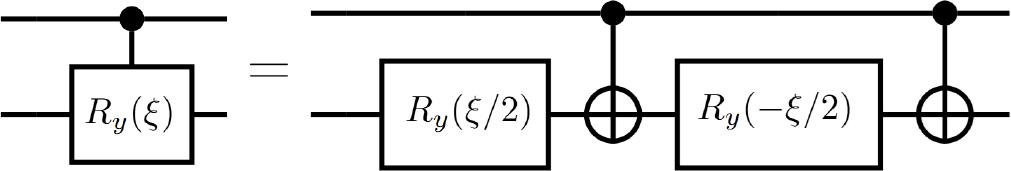
Representation of CRy gate using only basic gates
Additionally, the
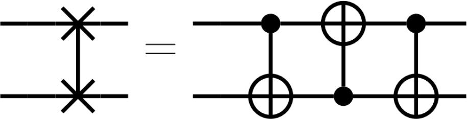
Representation of SWAP gate using only basic gates
Two sequential operators CRy and SWAP that are cR(u, v) and
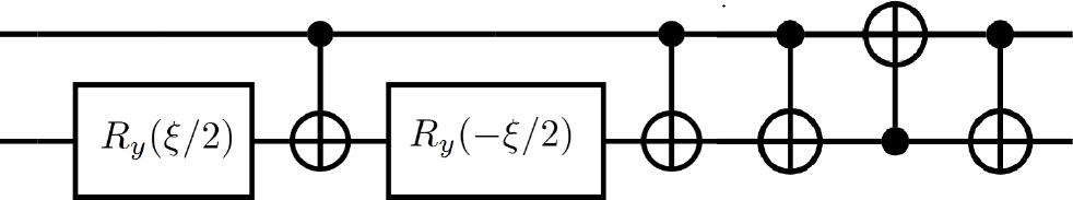
Representation of a pair CRy and SWAP gates using only basic gates
Note that two sequential
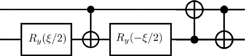
Reduced representation of a pair CRy and SWAP gates using only basic gates
Let us look at the CNOT cost of these operators, where the CNOT cost is the number of CNOT operators in the representation of a circuit using only basic gates.
We can say that the CNOT cost of cR(u, v) is 2; CNOT cost of
Finally, we can discuss the CNOT cost of the constructed circuit.
CNOT cost of the circuit generated by Algorithm 5 is 3k – 4b – 5 ≤ 3k – 5, where k is the length of a shortest non-simple path P = (vi1, …, vik) in the graph G that visits all vertices at least once, and b is the number of indices j such that vij = vij+2.
If we look at Algorithm 5, then we can see that it is a sequence of one of three options:
a pair of CRy and SWAP gates if vj ≠ vj+2 and vj+1 ∉ U.
SWAP gate if vj ≠ vj+2 and vj+1 ∈ U.
CRy gate if vj = vj+2 and vj+1 ∉ U.
Note that the option vj = vj+2 and vj+1 ∈ U is not possible because vj+1 ∈ U means that the corresponding qubit was already visited. In that case, we can just exclude it from the path because vj = vj+2. At the same time, it contradicts the condition that P is the shortest path.
The CNOT cost for pairs of CRy and SWAP gates is 3; for the SWAP gate, it is 3; for the CRy gate, it is 2.
Let b be the number of steps where we apply pairs of CRy and SWAP gates or the SWAP gate, and let b be the number of steps where we apply CRy (here we do not count the first and the last vertex from the path because they are processed by the different logic). Here a + 2b = k – 3 because (i) if vj = vj+2, then we use only CRy to vj+1 and skip vj+2 (ii) we do not count the target qubit. So, the total number of CNOT gates is 3a + 2b + 4 = 3(a + 2b + 3) – 4b – 5 = 3k – 4b – 5.
Using Lemma 3 we can estimate the CNOT cost of the circuit and present it in the next corollary.
CNOT cost of the circuit that is generated using Algorithm 5 is between 2n – 2 and 6n – 11.
The circuit has the minimal CNOT cost if each operation required only two CNOT gates, which means no SWAP gates. This happens if we have a “star” graph, where one vertex (a middle vertex) is connected to all other n – 1 vertices. In that case k = 2(n – 1) – 1 = 2n – 3, we start from a non-middle vertex and come to the middle vertex after each other, except the last one. The value b = n – 3 because each non-middle vertex, except the first and last in the path satisfies the required property. So, the CNOT cost according to Theorem 4 is 3(2n – 3) – 4(n – 3) – 5 = 6n – 9 – 4n + 12 – 5 = 2n – 2.
The maximum value is for k = 2n – 1, and the minimum value for b = 0. So, the maximum value for the CNOT cost is 3(2n – 1) – 5 = 6n – 6 – 5 = 6n – 11.
Typically, the quantum fingerprinting (quantum hashing) algorithm is used several times. For example, for hashing a string of ℓ symbols, we should apply the algorithm ℓ times (see Appendix B for examples). For this reason, we suggest two strategies.
Let a step be a single application of the quantum fingerprinting algorithm. After each step, we reverse the path P. Then, the target qubit travels back. Additionally, we can see that the operator
CNOT cost of the circuit to apply the quantum fingerprinting (quantum hashing) algorithm ℓ times is at most (3k – 4b – 7)ℓ + 2 ≤(3k – 7)ℓ + 2, where k is the length of the shortest non-simple path P = (vi1, …, vik) in the graph G that visits all vertices at least once, and b is the number of indices j such that vij = vij+2.
The first step costs 3k – 5 due to Theorem 4. Each next step skips the first
Similarly to Corollary 1 we can show the next result.
The CNOT cost of the circuit for application of the quantum fingerprinting (quantum hashing) algorithm ℓ times is between (2n – 4)ℓ + 2 and (6n – 13)ℓ + 2.
At the beginning of each step, starting from the second one, we add
Therefore, we have the following CNOT cost for ℓ applications of the quantum hashing algorithm.
CNOT cost of the circuit for application of the quantum fingerprinting (quantum hashing) algorithm ℓ times is at most
The first step costs 3k – 4b – 5 due to Theorem 4. Each next step costs 3k – 4b – 3 because of two additional
The total cost is
Due to b ≥ 0, we have
Similarly to Corollary 1 we can show the next result.
The CNOT cost of the circuit for application of the quantum hashing (quantum fingerprinting) algorithm ℓ times is between
Let us estimate the minimal cost similarly to Corollary 1. The first step costs 2n – 2. Each next step costs 2n – 2 + 2 = 2n. The total complexity is
Let us estimate the maximal cost similarly to Corollary 1. The first step costs 6n – 11. Each next step costs 6n – 11 + 2 = 6n – 9. The total complexity is
We can see that the complexity presented in Corollary 1 is less than the result from Corollary 3 because each cycle that visits all the vertices at least once can be converted to a path by removing the last edge. At the same time, the repeated application of the same pattern of gates for each step can be useful in some hardware implementations.
Let us compare our generic approach with existing circuits for specific graphs. The LNN architecture is a common layout graph for many quantum devices. The graph is a chain where v1 is connected with v2; vi is connected with vi–1 and vi+1 for i ∈ {2, …, n – 1}; vn is connected with vn–1.
The quantum fingerprinting (quantum hashing) algorithm for the LNN architecture was discussed in [79]. The path that visits all vertices in the graph is simply P = (v1, …, vn) (see Figure 7). So, our method gives us the same circuit as in [79]. The circuit for the quantum fingerprinting algorithm on 5 qubits is presented in Figure 8.
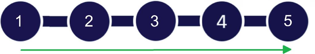
The graph for the 5-qubit LNN architecture. The path that visits all vertices at least once is green.
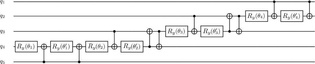
A quantum circuit for the Quantum hashing (quantum fingerprinting) algorithm for 5 qubits LNN architecture device.
The CNOT cost of the circuit is presented in the next lemma.
The CNOT cost of the produced circuit of the quantum fingerprinting (quantum hashing) algorithm with n qubits for the LNN architecture is 3n – 5 for one application and 3nℓ – 7ℓ + 2 for ℓ applications.
Let us consider more complex graphs like a cycle with tails (like a “sun” or “two joint suns”). The 16- and 27-qubit IBM machines of this architecture were considered in [23]. The graphs and paths are presented in Figures 9 and 10.
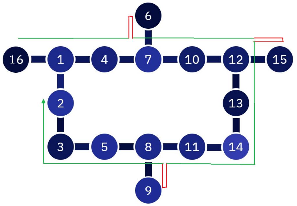
The graph for 16-qubit “sun” architecture. The path that visits all vertices at least once is green. Red parts are such that vij = vij+2.
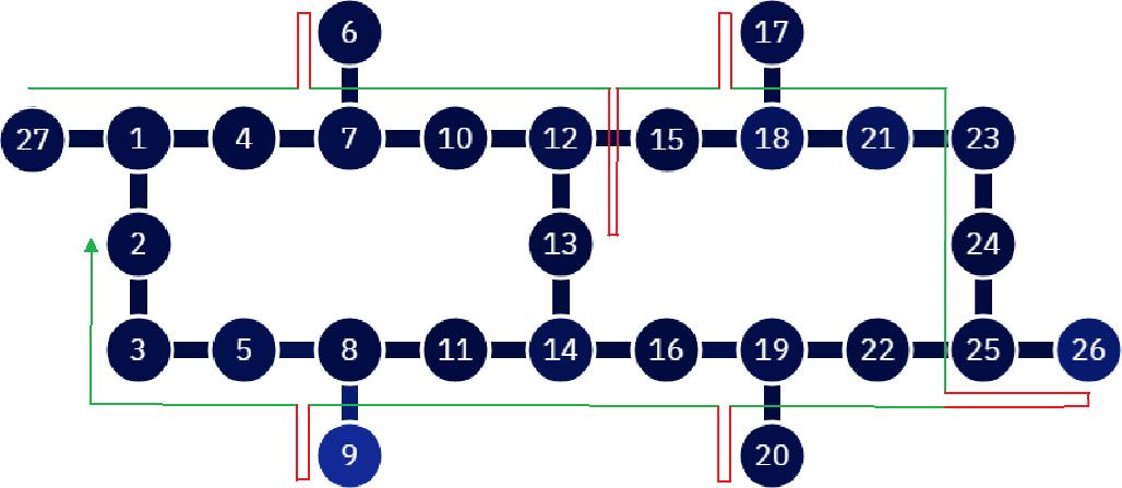
The graph for 27-qubit “two joint suns” architecture. The path that visits all vertices at least once is green. Red parts are such that vij = vij+2.
Note that the red part of the path is such that vj+2 = vj. Therefore, we do not apply a SWAP gate on this part of the path, but only a CRy gate. So, our generic method gives the same circuits as the circuits specially constructed for these devices [23]. The CNOT cost is 40 for the 16-qubit architecture, and 69 for the 27-qubit one.
We collect the results for the discussed architectures in Table 1 for LNN and Table 2 for others. Additionally, we added results in Table 3 for connectivity graphs of IBMQ Melbourne, Rigetti Aspen-4, and a 5 × 5-grid as a connectivity graph that can be found, for example, in [102]. They are presented in Figure 11.
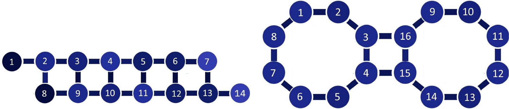
Connectivity graphs of IBMQ Melbourne, Regetti Aspen-4, and 5 × 5-grid.
The CNOT cost for the LNN architecture. The CNOT cost of circuits produced by algorithms from [79] and this paper is 3n – 5
| The number of qubits n | [79] and this paper | Qiskit transpiler |
|---|---|---|
| 5 | 10 | 14 |
| 10 | 25 | 39 |
The CNOT cost for “sun” and “two joint suns” architectures
| Connectivity graph’s type | [23] and this paper | Qiskit transpiler |
|---|---|---|
| 16-qubit “sun” architecture | 40 | 57 |
| 27-qubit “two joint suns” architecture | 69 | 115 |
The CNOT cost for IBMQ Melbourne, Regetti Aspen-4, and 5 × 5-grid
| Connectivity graph’s type | This paper | Qiskit transpiler |
|---|---|---|
| 14-qubit IBMQ Melbourne | 36 | 44 |
| 16-qubit Regetti Aspen-4 | 43 | 66 |
| 25-qubit 5 × 5-grid | 70 | 84 |
Moreover, we compare our algorithm with Qiskit transpiler [103] optimized circuit for the mentioned architectures. The Qiskit’s algorithm is randomized heuristic algorithm for circuit optimization. That is why we invoke it 100 times and choose the minimum of the produced circuits’ CNOT costs. We added the results to the tables.
The results were obtained using the algorithm implemented in C++. The implementation can be found in GitLab repository [104].
In this paper, we focus on the CNOT cost (the number of CNOT gates) because two-qubit gates are harder to implement on real devices and give larger computational error compared to one-qubit gates. At the same time, there is another common metric of circuit quality that is depth (the number of steps, where each step is a layer of gates that can be done in parallel on different qubits). Often, the depth of a circuit is associated with time complexity. We do not optimize this metric in this paper. However, if we compute the depth of the circuit, then it can be obtained from the CNOT cost by adding 2(n – 1) because we do n – 1 controlled rotations in total and each of them requires two rotation gates as shown in Figure 3.
Here we present a method that allows us to construct a circuit for the Quantum Fourier Transform (QFT) for a connected graph G = (V, E) that is a qubit connectivity graph for a device. More information about the QFT algorithm can be found in Appendix C. If we do not have restrictions for applying two-qubit gates (when G is a complete graph for instance), then the circuit is as presented in Figure 12.
A quantum circuit for the Quantum Fourier Transform algorithm for fully connected 5 qubits.
The author of [23] shows that the circuit for QFT is a series of CNOT cascades. Each of the cascades has a gate structure similar to the shallow circuit for the quantum hashing algorithm. Assume that we have a C
Let us present the whole algorithm for constructing the quantum circuit for the QFT algorithm.
Firstly, we find a non-simple path P = (vi1, …, vjk) that visits all vertices at least once. Then we assign logical qubits to the vertices according to this path. Let indices j1, …, jn be the indices of the first occurrence of each vertex. In other words, jr is such that ijr = r, and ih ≠ r for each 1 ≤ h < jr.
Then, we assign Qr ← jr the position of r-th logical qubit in the graph, and Tjr ← r the index of the logical qubit associated with a vertex.
After that, we start to construct the circuit for cascades. For the first cascade, we invoke C
For the second cascade, we exclude the vertex with index Q1 from the graph and find the path P′ that visits all vertices at least once in the updated graph such that it starts from the vertex vQ2. The vertex vQ2 contains the 2nd logical qubit that should be the target in the second cascade. Then, we invoke C
For the next cascades, we act in a similar way. For the r-th cascade, we exclude vQr–1, find the path P′ that visits all vertices at least once in the updated graph such that it starts from the vertex vQr, and invoke C
Note that a path in the updated graph always exists because it is connected. We have at least one path that visits all vertices at least once, and we exclude only one vertex, that is, the last one on this path.
During the implementation, we do not remove the vertex from the graph; we just store a set of “deleted” vertices and we prohibit visiting vertices from this set during the algorithm for the path search.
Let us present the algorithm.
- Step 1.
We find a non-simple path P = (vi1, …, vik) that visits all vertices at least once.
- Step 2.
We find indices j1, …, jn, where jr is such that ih ≠ ijr for each 1 ≤ h < jr. Then, we assign Qr ← jr and Tijr ← r for 1 ≤ r ≤ n.
- Step 3.
We assign P′ ← P, and k′ is the length of P′. We assign r ← 1, which is an index of the cascade.
The next steps are repeated while the graph contains at least one vertex.
- Step 4.
We find a non-simple path P′ of length k′ that visits all non-deleted vertices of the graph and starts from vQr. If r = 1, then we do nothing because P′ was already found in Steps 1-3.
- Step 5.
We invoke C
onstruct QFTFor Path (P′, k′, r), which is the r-th cascade. Assume that the procedure keeps the Q and T indices actual. - Step 6.
We exclude vQr from the graph.
- Step 7.
If r = n, then we terminate the algorithm. Otherwise, we increase the index of the cascade r ← r + 1 and go to Step 4.
The implementation of the algorithm is presented in Algorithm 6. Assume that we have the Sh
P ← S
(j1, …, jn) ←
for r ∈ {1, …, n} do
Qr ← jr
Tijr ← r
end for
P′ ← P, k′ ← k, r ← 1
while r ≤ n do
C
V ← V\{vQr}
r ← r + 1
if r ≤ n then
P′ ← S
end if
end while
Let us discuss the time complexity of the algorithm. The time complexity of S
The procedure C
- Step 1.
We start with the first qubit in the path j ← 1. We apply the Hadamard transformation to the qubit corresponding to the vertex vi1. We denote this action by H(vi1). If k′ = 1, then we terminate our algorithm; otherwise, go to Step 2.
- Step 2.
If j = k′, then we terminate the algorithm; otherwise, we continue. If vij+1 ∉ U, then we apply the controlled phase gate CRd with the control vij+1 and the target vij. qubits, where d = Tij+1 – r. Then, we add vij+1 to the set U, i.e., U ← U ∪ {vij+1 }. Then, we go to Step 3.
- Step 3.
If j = k′ – 1 or vij+2 ≠ vij, then we continue; otherwise, we go to Step 4. We apply the SWAP gate to vij and vij+1, and swap the indices of qubits for these vertices. In other words, if w1 = Tij and w2 = Tij+1 are indices of the corresponding logical qubits, then we swap Qw1 and Qw2 values, and Tij and Tij+1 values. Then, we update j ← j + 1 because the value of the target qubit moves to vij+1. Then, we go to Step 2.
- Step 4.
If vij+2 = vij, then we update j ← j + 2. Note that here we stay on the same vertex of the graph G. Then, we go to Step 2.
Finally, we obtain C
j ← 1 ▷Step 1
H(vij)
U ← ∅
while j ≤ k′ do ▷Step 2
if vij+1 ∉ U then
d ← Tij+1 – r
CRd(vij+1, vij)
U ← U ∪{vij+1}
end if
if j = k′ or vij+2 ≠ vij. then ▷Step 3
if k′ = 2 then
w1 ← Tij, w2 ← Tij+1
Qw1 ← ij+1, Qw2 ← ij
Tij ← w2, Tij+1 ← w1
end if
j ← j + 1
else ▷Step 4
j ← j + 2
end if
end while
Let us start with discussion correctness of the algorithm.
The quantum circuit produced by Algorithm 6 implements the circuit of the quantum Fourier transform algorithm from Figure 12.
The r-th cascade of the QFT circuit is such that we should apply controlled phase operators with each logical qubit with indexes larger than r as the control qubit and r-th qubit as the target.
For the cascade, the algorithm computes the path that starts from the vertex corresponding to the r-th logical qubit and visits all vertices corresponding to the logical qubit with indexes larger than r. Let the path be
So, if the target qubit is in vij, then we apply the controlled phase operator with vij+1 as the control qubit and move the target qubit to vij+1 using the swap gate.
We apply the controlled rotation phase with vij+1 as the control qubit only if it is not in the set U, and then add it to the set U. This action guarantees us that we apply the controlled phase operator with each required qubit only once. At the same time, the path visits each vertex corresponding to logical qubits with indexes larger than r at least once. This means that each qubit (vertex) occurs as vij+1 for some j. So, we apply the controlled phase operator with each qubit exactly once, and there are no other modifications of the target qubit. Therefore, the circuit implements the r-th cascade.
After that we exclude the vertex corresponding to r-th logical qubit from the graph. Note that the rest of the graph is connected because the r-th logical qubit moved to the end of the path P′. So, we can be sure that all vertices corresponding to logical qubits with indexes larger than r are connected with path P′ without the last vertex. Therefore, we can repeat the algorithm for the next cascades.
So, the produced circuit implements all cascades of the QFT circuit presented in Figure 1. At the same time, we apply the swap or controlled phase operators only to neighboring qubits.
Let us continue with CNOT cost of the circuit.
Note that the CRd gate can be represented using only two CNOT gates and three Rz gates similar to CRy [105] (see Figure 13).
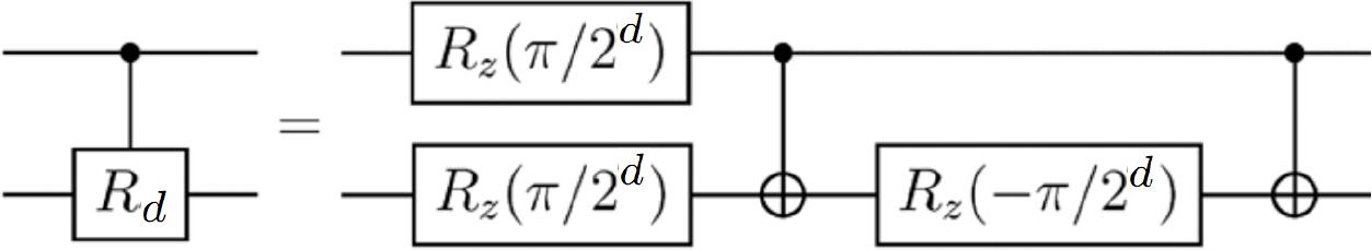
Representation of CRd gate using only basic gates.
A pair CRd and SWAP can be represented using three CNOT gates. (See Figure 14).
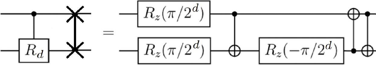
Reduced representation of a pair Rd and SWAP gates using only basic gates.
If the graph G with n vertices has a Hamiltonian path, then the CNOT cost of the produced circuit for the QFT algorithm is 1.5n2 – 1.5n – 1.
Because the graph has a Hamiltonian path, the path P = (vi1, …, vin) is exactly this path. So, in each step, we move the target qubit. We can say that in constructing the r-th cascade, we use the path P′ = (vi1, …, vin–r+1). The CNOT cost of the r-th cascade for 1 ≤ r ≤ n – 2 is 3(n – r) because we apply SWAP and the controlled phase gates for each edge of the path. The CNOT cost of the (n – 1)-th cascade is 2 because we do not apply the SWAP gate. The CNOT cost of the n-th cascade is 0. Therefore, the total cost is
Let us discuss the CNOT cost of the algorithm in the next theorem.
The CNOT cost of a circuit that is generated using Algorithm 5 is between n2+ n – 4 and 3n2 – 3n – 10.
Similarly to Corollary 1, the minimal possible cost is when we move the target qubit the minimum possible times. It is the situation with the “star” graph where we have a vertex connected with all others. The cost of the r-th cascade in that case is 3 + 3 + 2 · (n – 2 – r) = 2(n – r) + 2, because we always remove one “non-middle” vertex. The path starts from “non-middle” and finishes in “non-middle.” Therefore, we should make two moves of the target qubit. For the (n – 1)-th cascade, the cost is only 2. So, the total complexity is at least
Similarly to the proof of Theorem 4, we can show that the CNOT cost of one cascade is at most 3(k – 1). After each cascade, the number of vertices is decreased by 1. The maximum possible value for k is 2n – 1. In the r-cascade, it is 2(n – r + 1) – 1 = 2(n – r) + 1. The cost of the (n – 1)-th cascade is 2, not 3, because we do not move the target qubit. The cost of the (n – 2)-th cascade is 6, because the length of the path in the graph with 3 vertices is always 3. So, the total complexity is at most
Similarly to Section 4.1 we discuss the LNN architecture and the more complex architecture. Firstly, let us consider the LNN architecture. As discussed earlier (see Figure 7), the path visits all vertices from v1 to vn one by one. The paths constructed for each cascade are presented in Appendix E. The circuit is similar to the circuit developed in [23]. The presented path is the Hamiltonian path in the graph. Due to Theorem 8, we get the following CNOT cost for the LNN architecture.
The CNOT cost of the produced circuit of the QFT algorithm using n qubits for the LNN architecture is 1.5n2– 1.5n – 1.
At the same time, [14] gives the circuit with n2 + n – 4 CNOT cost, and [23] gives the circuit with 1.5n2 – 2.5n + 1 CNOT cost. Our circuit is better than [14] only if n ≤ 3. The result from [23] is better than our result. However, it is not known how to apply the results of [14] for more complex architectures, and the results of [23] are presented only for a specific architecture.
Secondly, let us consider more complex architectures like 16-qubit “sun” (Figure 9), and 27-qubit “two joint suns” (Figure 10). The paths are presented in figures. Note that the red part of the path is such that vj+2 = vj. Therefore, we do not apply a SWAP gate on this step, but only the controlled phase operator. The CNOT cost for the 16-qubit machine is 342, and for the 27-qubit machine is 1009.
So, our generic method gives circuits that are a bit worse than the circuits constructed especially for these devices [23], which CNOT costs are 324 and 957 for the 16-qubit and the 27-qubit architectures, respectively. The difference is about 5%.
We have collected the results of discussed architectures in Table 4 for LNN and Table 5 for others. Additionally, we added results in Table 6 for connectivity graphs of IBMQ Melbourne, Rigetti Aspen-4, and a 5 × 5-grid as a connectivity graph that can be found, for example, in [102]. They are presented in Figure 11.
The CNOT cost of quantum circuit for the QFT algorithm for LNN architecture. The CNOT cost of circuits produced by the algorithm from [14] is n2 + n – 4; by the algorithm from [79] is 1.5n2 – 2.5n + 1; the algorithm from this paper is 1.5n2 – 1.5n – 1.
| The number of qubits n | This paper | [14] | [79] | Qiskit transpiler |
|---|---|---|---|---|
| 3 | 8 | 8 | 7 | 9 |
| 4 | 17 | 16 | 15 | 21 |
| 5 | 29 | 26 | 26 | 38 |
| 10 | 134 | 106 | 126 | 207 |
The CNOT cost of quantum circuit for the QFT algorithm for “sun” and “two joint suns” architectures
| Connectivity graph’s type | This paper | [23] | Qiskit transpiler |
|---|---|---|---|
| 16-qubit “sun” architecture | 342 | 324 | 549 |
| 27-qubit “two joint suns” architecture | 1009 | 957 | 1839 |
The CNOT cost of quantum circuit for the QFT algorithm for IBMQ Melbourne, Regetti Aspen-4, and 5 × 5-grid
| Connectivity graph’s type | This paper | Qiskit transpiler |
|---|---|---|
| 14-qubit IBMQ Melbourne | 269 | 335 |
| 16-qubit Regetti Aspen-4 | 359 | 585 |
| 25-qubit 5 × 5-grid | 899 | 1158 |
Moreover, we compare our algorithm with the Qiskit transpiler [103] optimized circuit for the mentioned architectures. The Qiskit’s algorithm is a randomized heuristic algorithm for circuit optimization. That is why we invoke it 100 times and choose the minimum of the produced circuits’ CNOT costs. We added the results to the tables.
The results were obtained using the algorithm implemented in C++. The implementation can be found in the GitLab repository [104].
As we discussed in Remark 2, here, we focus on the CNOT cost but not the depth of the circuit. If we compute the depth of the circuit, then it can be obtained from the CNOT cost by adding n2 because for r-th cascade we do n – r controlled phase gates in total and each of them required two additional layers for rotation gates as shown in Figure 13. Moreover, we add one H gate. So, the depth of the r-th cascade is 2(n – r) + 1. The total depth is
We present a generic method for constructing quantum circuits for quantum fingerprinting (quantum hashing) and quantum Fourier transform algorithms for an arbitrary connected qubit connectivity graph for hardware. The heuristic version of the method is fast enough and works with O(n6) time complexity. The certain version has an exponential time complexity that is O(n22n). The algorithm works for an arbitrary qubit connectivity graph.
At the same time, if we consider samples of graphs like LNN, “sun” (16-qubit IBMQ Eagle r3 architecture), “two joint suns” (27-qubit IBMQ Eagle r3 architecture), then our generic algorithm gives us the same circuit as the techniques provided especially for these graphs [23,79] in the case of quantum hashing. In the case of QFT, our algorithm gives a bit worse circuit compared to the techniques optimized for these graphs [14,23]. At the same time, our approach works for arbitrary connected graphs, but the existing results work only for some specific graphs. Additionally, we consider other different architectures like IBMQ Melbourne, Rigetti Aspen-4, and a 5 × 5-grid as a connectivity graph. We show that for all of the considered connectivity graphs, including LNN, “sun,” and “two joint suns,” our algorithm produces circuit better than standard Qiskit transpiler optimization.
An open question is to develop a technique for QFT for an arbitrary connected graph that gives us the same or better results than the existing ones for specific architectures like LNN, “sun” and “two joint suns.”