
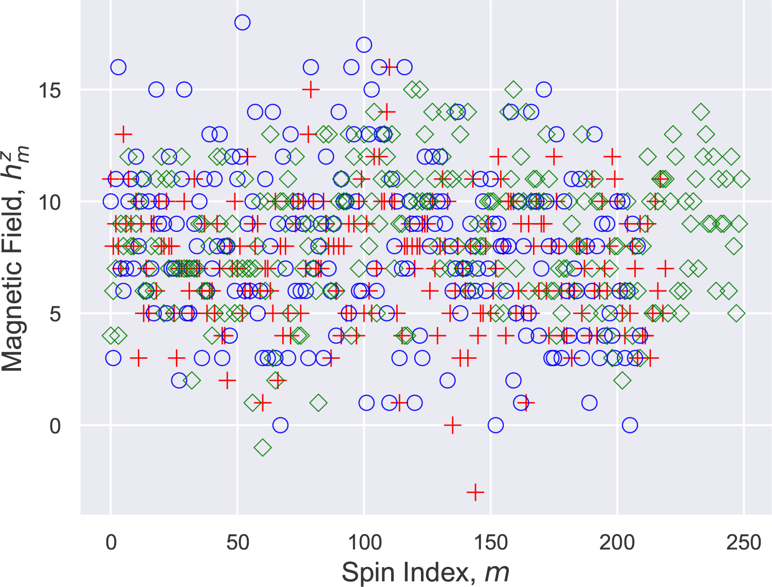
Figure 1.
The spin representations of three Sudoku puzzles published in The New York Times on January 2 (diamond), January 12 (circle), and January 14 (plus), 2025, are shown. The mean and standard deviation of the magnetic field are as follows: 8.7 ± 3.0 for the January 2 puzzle (diamond), 8.0 ± 3.7 for January 12 (circle), and 7.3 ± 2.7 for January 14 (plus).
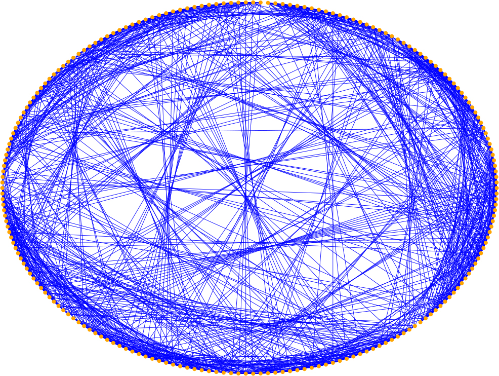
Figure 2.
The dense, long-range couplings among the 210 spins for the January 12, 2025, Sudoku puzzle. Each line represents an Ising coupling Jm,n = 2, which favors spin-m and spin-n being antiparallel. Each spin can point either up or down. Finding the lowest-energy spin configuration corresponds to solving the Sudoku puzzle.
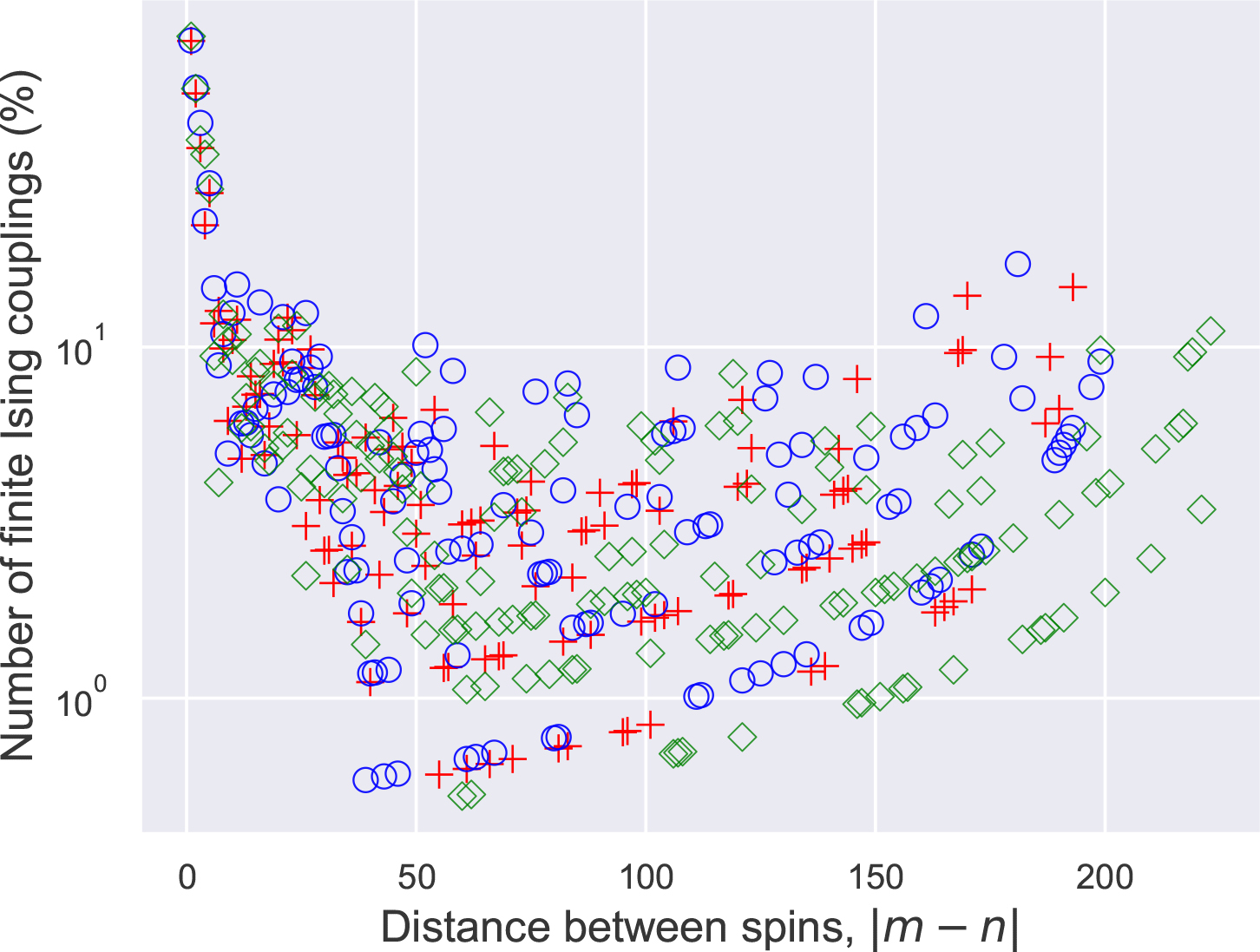
Figure 3.
Statistical analysis of the couplings between the spins. For nearest neighbors, about 75% are coupled. The coupling fraction drops to the 10% level when the distance grows to 6 or 7, then fluctuates between 1% and 10%. The legends are the same as Figure 1. The vertical axis is in logarithmic scale.
Table 1.
A few examples of solved Sudoku puzzles in chronological order according to their publication date in The New York Times. These puzzles vary in the number of clues (Nc), total number of spins (Ns), and other parameters; see the main text for details.
| Puzzle date | Level | Nc | N↑ | Ns | c1+c2+c3 |
|---|---|---|---|---|---|
| January 8, 2024 | h | 24 | 57 | 211 | 368.5 |
| December 10, 2024 | m | 26 | 55 | 200 | 359.0 |
| January 2, 2025 | m | 22 | 59 | 250 | 520.5 |
| January 8, 2025 | m | 23 | 58 | 232 | 461.5 |
| January 12, 2025 | m | 27 | 54 | 210 | 426.5 |
| January 14, 2025 | m | 23 | 58 | 232 | 457.0 |
| January 15, 2025 | m | 25 | 56 | 210 | 380.0 |
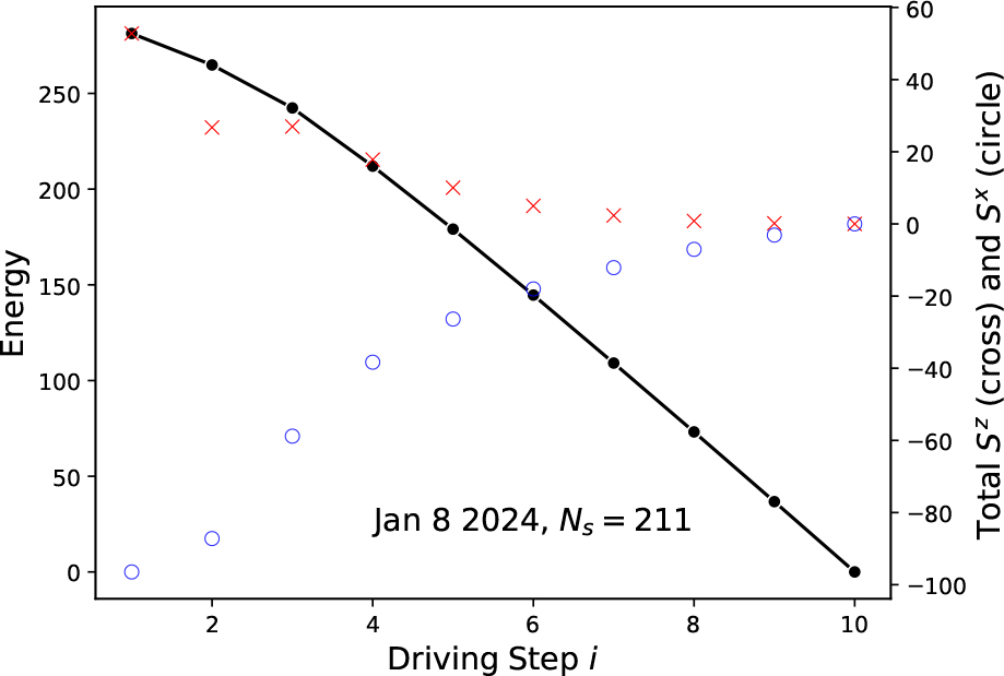
Figure 4.
How the January 8, 2024, puzzle gets solved: As the driving field hx is reduced, the energy gradually drops to zero. The total spin along the x-direction vanishes, while the total spin along the z-direction approaches its ground state value. The bond dimension is D = 20, and the driving field is set to hx = 0.75.
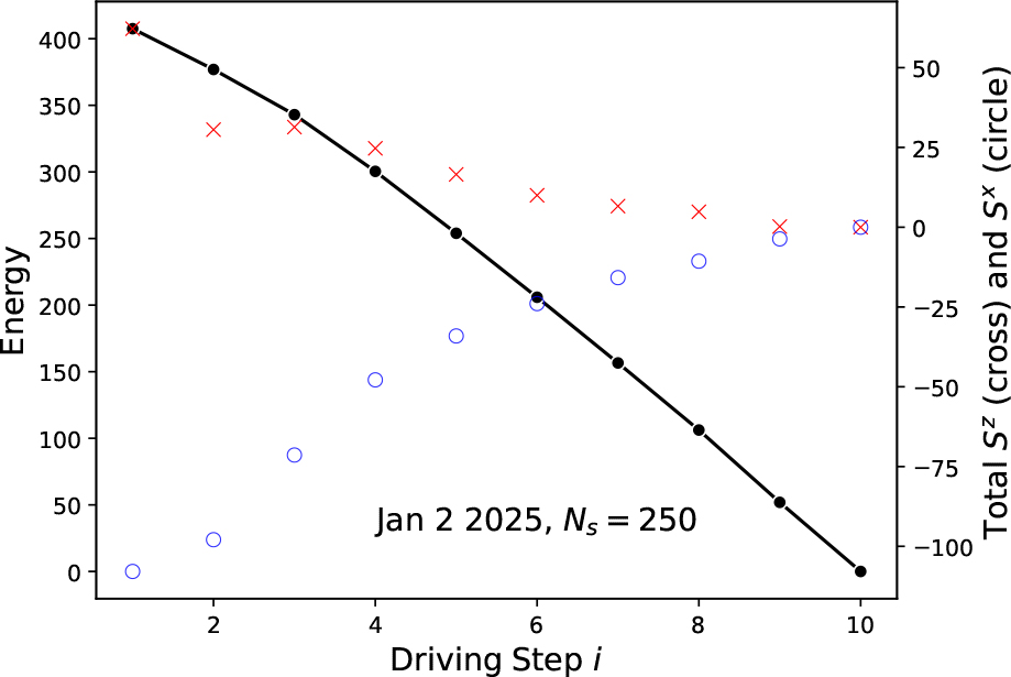
Figure 5.
The solution process for another puzzle with fewer clues and more spins: D = 20, hx = 1.
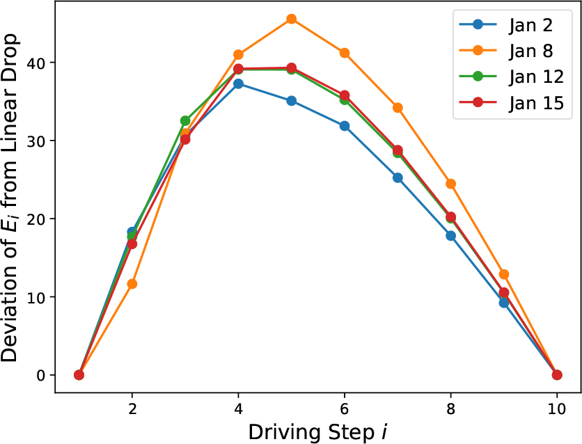
Figure 6.
The nonlinear drop in energy during the driving process. See main text for details.
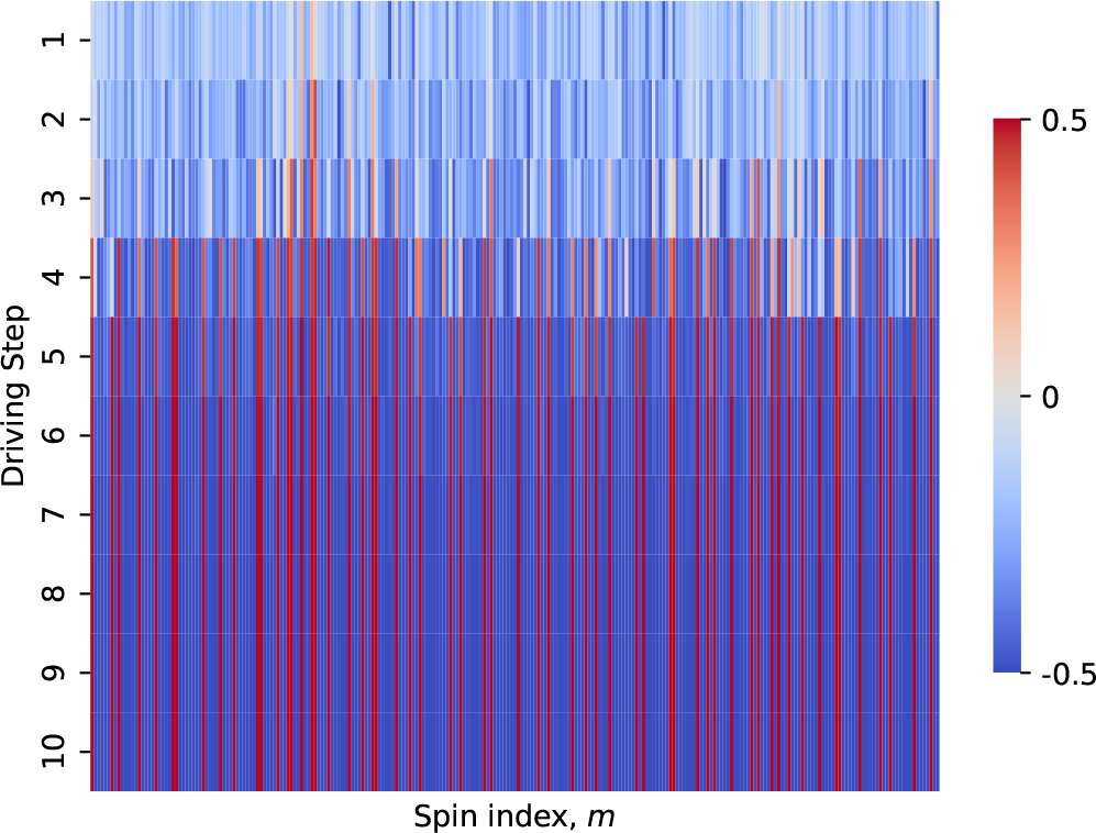
Figure 7.
The evolution of the 251 spins during the solution process of the January 2, 2025, puzzle. The value of is color-coded: red represents spin-up, and blue represents spin-down.
Table 2.
Twenty weighted MaxCut instances and the parameters used to solve them. Each instance is identified by its file name in the Biq Mac Library. The edge weights are either 1 or – 1. For the first ten instances, the number of vertices NV = 80 and the number of edges NE = 316. For the next ten instances, NV = 100 and NE = 495. The algorithm successfully finds E0, the ground state energy of the spin model (the MaxCut value is simply – E0), except for the case pm1s_100.5.
| Instance | E0 | M | hx | η | D |
|---|---|---|---|---|---|
| pm1s_80.0 | –79 | 5 | 1 | 0 | 30 |
| pm1s_80.1 | –69 | 5 | 1 | 0 | 30 |
| pm1s_80.2 | –67 | 5 | 1 | 0.3 | 30 |
| pm1s_80.3 | –66 | 5 | 1 | 0 | 30 |
| pm1s_80.4 | –69 | 5 | 1 | 0.3 | 30 |
| pm1s_80.5 | –66 | 20 | 1 | 0.3 | 30 |
| pm1s_80.6 | –71 | 5 | 1 | 0 | 30 |
| pm1s_80.7 | –69 | 5 | 1 | 0 | 30 |
| pm1s_80.8 | –68 | 5 | 1 | 0 | 30 |
| pm1s_80.9 | –67 | 5 | 1 | 0 | 30 |
| pm1s_100.0 | –127 | 5 | 1 | 0.3 | 30 |
| pm1s_100.1 | –126 | 5 | 1 | 0.3 | 30 |
| pm1s_100.2 | –125 | 10 | 1 | 0.3 | 30 |
| pm1s_100.3 | –111 | 10 | 1 | 0.3 | 30 |
| pm1s_100.4 | –128 | 5 | 1 | 0.3 | 30 |
| pm1s_100.5 | –125 | 10 | 1 | 0 | 60 |
| pm1s_100.6 | –122 | 10 | 1 | 0.3 | 30 |
| pm1s_100.7 | –112 | 20 | 1 | 0.3 | 60 |
| pm1s_100.8 | –120 | 10 | 1 | 0.3 | 30 |
| pm1s_100.9 | –127 | 5 | 1 | 0.3 | 30 |
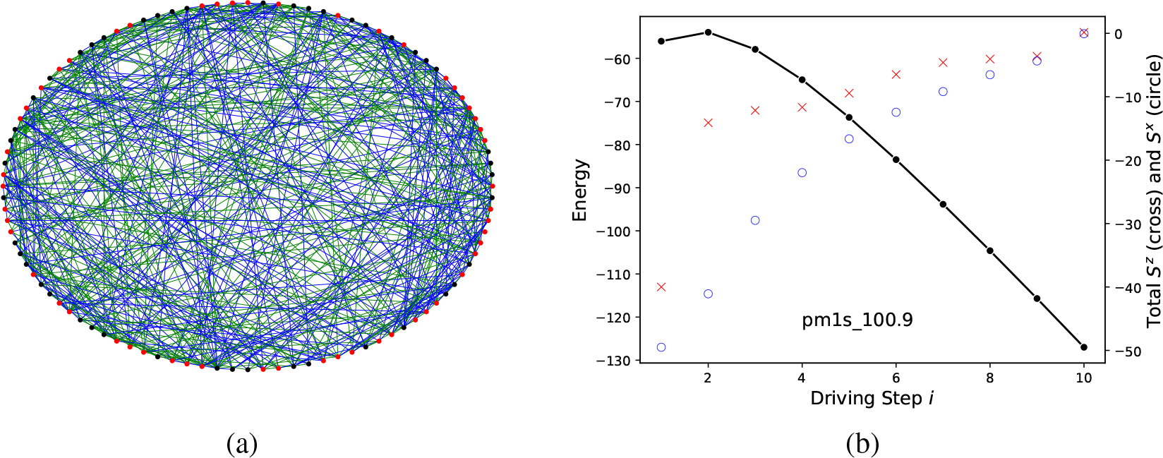
Figure 8.
(a) Graph representation of the problem. The edges carry weights of 1 (in green) or – 1 (in blue). The solution is indicated by the node color: nodes in black belong to set A, while the rest of the nodes (in red) belong to set Ā. (b) The energy (dot), expectation values of Sz (cross, measured from its ground state value and magnified by 10 times), and Sx (circle) during the driving process. Solving the weighted MaxCut instance pm1s_100.9 from the Biq Mac Library.
Table 3.
Twenty unweighted MaxCut instances from the Biq Mac Library with dense edges. The first ten cases have NV = 60 and NE = 885, while the remaining cases have NV = 100 and NE = 2,475. All edge weights are set to 1. The algorithm successfully solves all instances except g05_100.3 and g05_100.5, where the E0 values should be – 1,424 and – 1,436, respectively [39,40]. Here, Nsw refers to the number of DMRG sweeps per driving step, with hx = 1 and η = 0.3.
| Instance | E0 | M | Nsw | D |
|---|---|---|---|---|
| g05_60.0 | –536 | 10 | 5 | 30 |
| g05_60.1 | –532 | 10 | 5 | 40 |
| g05_60.2 | –529 | 10 | 5 | 30 |
| g05_60.3 | –538 | 10 | 5 | 30 |
| g05_60.4 | –527 | 10 | 5 | 30 |
| g05_60.5 | –533 | 10 | 5 | 30 |
| g05_60.6 | –531 | 10 | 5 | 30 |
| g05_60.7 | –535 | 10 | 5 | 60 |
| g05_60.8 | –530 | 10 | 5 | 30 |
| g05_60.9 | –533 | 20 | 5 | 40 |
| g05_100.0 | –1430 | 20 | 5 | 40 |
| g05_100.1 | –1425 | 20 | 5 | 40 |
| g05_100.2 | –1432 | 20 | 5 | 40 |
| g05_100.3 | –1423 | 10 | 5 | 30 |
| g05_100.4 | –1440 | 20 | 5 | 40 |
| g05_100.5 | –1435 | 10 | 5 | 30 |
| g05_100.6 | –1434 | 10 | 10 | 40 |
| g05_100.7 | –1431 | 10 | 10 | 40 |
| g05_100.8 | –1432 | 10 | 10 | 60 |
| g05 100.9 | –1430 | 10 | 10 | 40 |
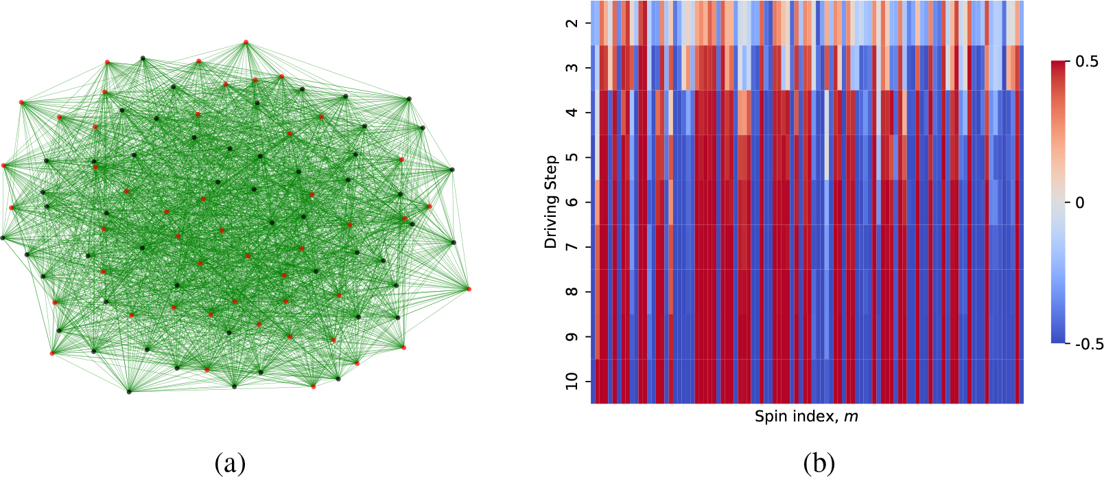
Figure 9.
(a) Graph representation of the problem. All edges (green lines) carry equal weight of 1. The MaxCut found by our algorithm is color-coded: nodes in black belong to set Ā, while nodes in red belong to set Ā. (b) The expectation value of during the driving process as the spins gradually settle into their ground state orientation (red represents spin up, blue represents spin down). Only driving steps 2 to 10 are shown to enhance the color contrast. Solving the unweighted MaxCut instance g05_100.4 from the Biq Mac library.
Table 4.
The algorithm parameters used to successfully solve five MaxCut instances from the Biq Mac Library with 251 vertices and over 3200 edges, each with integer weights; D = 30, M = 10.
| Instance | E0 | NV | NE | hx | η | Nsw |
|---|---|---|---|---|---|---|
| bqp250-2 | -44810 | 251 | 3285 | 0.05 | 0 | 10 |
| bqp250-4 | -41274 | 251 | 3397 | 0.05 | 0 | 10 |
| bqp250-6 | -41014 | 251 | 3433 | 0.30 | 0 | 5 |
| bqp250-8 | -35726 | 251 | 3265 | 0.05 | 0 | 10 |
| bqp250-10 | -40442 | 251 | 3294 | 1.00 | 0.3 | 5 |
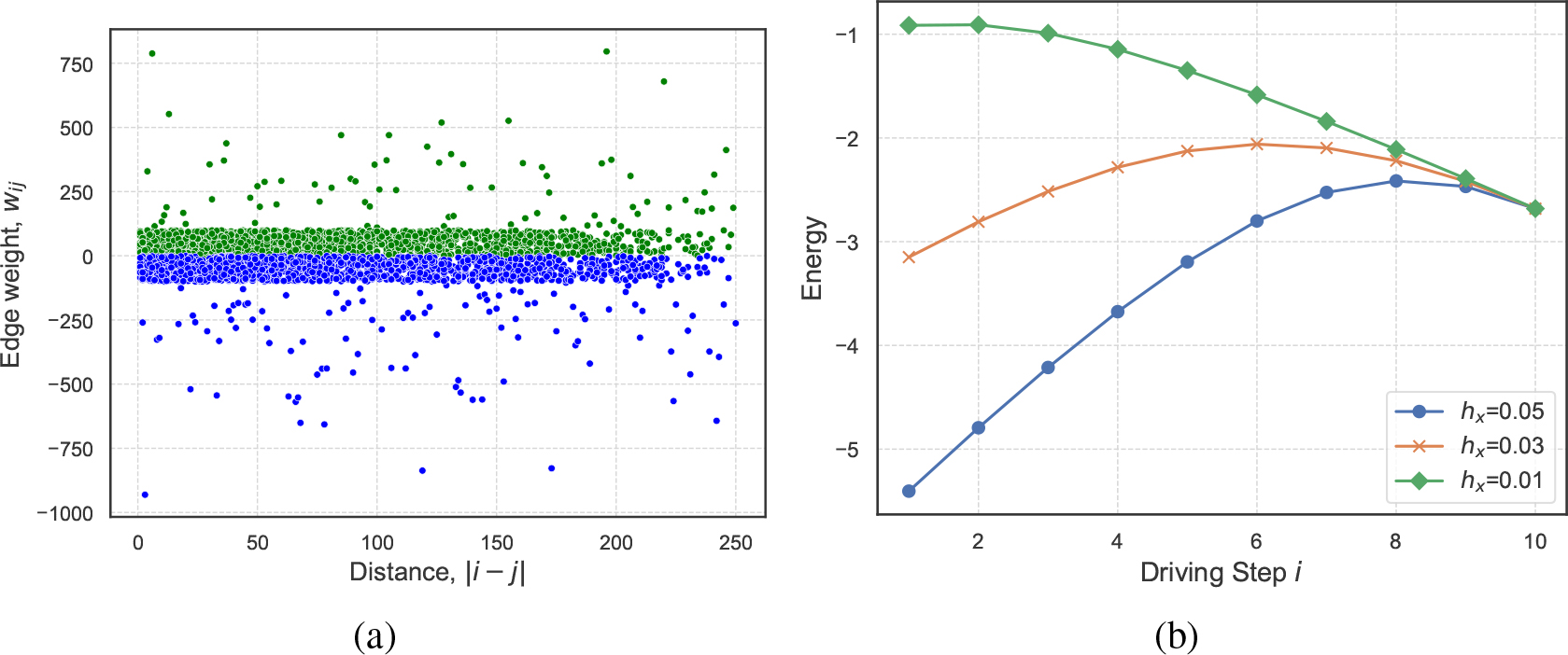
Figure 10.
(a) The distribution of the edge weights wi,j sorted by |i – j|, the distance between the nodes. Most of the weights lie within the interval from –100 to 100. (b) The variation of energy during the driving process for three different values of hx. All three choices converge to the ground state, yielding the correct MaxCut value. The edge matrix has been normalized such that the maximum absolute value of its elements is 1. Solving MaxCut instance bqp250-8 with 251 nodes and 3265 edges.