
Combinatorial optimization problems are both fundamentally important and computationally challenging [1,2]. They arise in a wide range of industries, including logistics, supply chain management, vehicle routing, drug discovery, and portfolio optimization. Classical problems such as the traveling salesman problem have played a pivotal role in shaping the field of computational complexity theory [3]. A broad class of these optimization problems can be reformulated as Quadratic Unconstrained Binary Optimization (QUBO) problems [4,5], which admit a compact mathematical representation:
A common strategy in quantum optimization algorithms is to encode the objective function into a cost Hamiltonian Hc, which is then manipulated using quantum superposition, tunneling, and other non-classical effects [7]. Since the variables xi are binary, a QUBO problem can be naturally mapped onto an Ising-type spin (or qubit) Hamiltonian [8,9]. In this mapping, the QUBO matrix Q defines the Ising couplings, and the cost function f corresponds to the eigenvalues of Hc. Thus, solving the optimization problem becomes equivalent to finding the ground state of Hc. In quantum annealing [10–12], a driver Hamiltonian that does not commute with Hc is introduced. The system is initialized in the ground state of the driver Hamiltonian—typically an equal-weight superposition over all computational basis states—and is then evolved adiabatically as the driver strength is gradually decreased and the cost Hamiltonian is amplified. Under ideal conditions, the system remains in its instantaneous ground state throughout this process, eventually reaching the ground state of Hc, which encodes the optimal solution. The Quantum Approximate Optimization Algorithm (QAOA) [13,14] takes a different approach by applying alternating layers of unitary transformations—referred to as cost and mixer layers—to a set of qubits initialized in some superposition state. After each iteration, the expectation value of the cost Hamiltonian is measured, and a classical optimizer updates the variational parameters to maximize performance. This hybrid quantum-classical loop is repeated until a set of parameters is found that yields a high-quality solution [14]. In our quantum-inspired algorithm, we adopt the concepts of driver and mixer Hamiltonians to guide the optimization process in a purely classical framework.
The practical implementation of quantum algorithms is currently constrained by the limitations of available hardware. For example, in the D-Wave Advantage annealer, each qubit can couple with at most 15 other qubits [15], whereas many QUBO problems require denser or long-range connectivity. Similarly, the applicability of QAOA is limited by qubit coherence times and circuit depth, restricting its use to relatively small systems with up to approximately 40 qubits [16,17]. These hardware constraints have spurred interest in quantum-inspired algorithms, which do not rely on quantum hardware but instead simulate certain quantum behaviors—such as superposition and tunneling— on classical machines. By emulating these features, quantum-inspired approaches have demonstrated the potential to outperform traditional classical heuristics on a variety of optimization problems [18–21].
In this work, we propose and evaluate a quantum-inspired algorithm for solving QUBO problems involving over 200 variables with dense connectivity. To benchmark its performance, we focus on problem instances where the optimal solution is challenging to find but straightforward to verify. Although many curated optimization problems exist, the global optimum is often unknown or unproven for medium-to large-scale instances. This limitation motivates our choice of a well-established class of problems that admit QUBO formulations, offer multiple variants, and critically have easily verifiable solutions: Sudoku puzzles.
This work is motivated by a simple question: Can quantum mechanics help solve Sudoku puzzles? Although Sudoku can be formulated as a QUBO problem, it appears to be beyond the practical reach of current quantum optimization methods. For instance, Mücke [22] reports that quantum annealing was unable to reliably find the correct solution (see Figure 4 in [22]), and QAOA has not demonstrated success on such instances. In this sense, Sudoku puzzles represent a kind of “worst-case scenario” for QUBO problems: the cost function is entirely constraint-driven, with non-local dependencies involving many binary variables. Once the puzzle’s clues are incorporated, the resulting Ising model exhibits long-range couplings and an inhomogeneous on-site magnetic field—features that make the spin landscape highly complex and challenging to optimize. Moreover, Sudoku provides an exacting benchmark: the solution is easy to verify, but correctness demands that the algorithm locate the exact ground state. Merely reducing the energy or producing a partially correct board is insufficient. As such, success requires not just approximate optimization but full satisfaction of all constraints. This makes Sudoku puzzles an ideal testbed for assessing the reliability and quality of a QUBO solver.
We emphasize that the goal of this work is not to develop a Sudoku solver that outperforms classical methods. Indeed, Sudoku can be solved manually, or via efficient classical algorithms such as backtracking, constraint propagation, or simulated annealing applied to its QUBO formulation. Rather, our interest in Sudoku lies in its ability to generate hard, structured QUBO problems that have proven challenging for quantum and quantum-inspired approaches. Once our algorithm successfully passes this stringent test, we extend its application to a range of MaxCut problems. Although MaxCut instances differ in structure from Sudoku, the algorithm continues to perform well, consistently finding optimal solutions.
A central innovation of our approach is the combination of a discrete driving schedule with a sweeping procedure applied to the many-spin wavefunction. Specifically, we adapt techniques from quantum many-body physics, borrowing the concepts of Matrix Product States (MPS) [23] and the Density Matrix Renormalization Group (DMRG) algorithm [24,25], both of which originate in the study of low-dimensional quantum systems [26]. While MPS and DMRG were originally developed for one-dimensional systems with local interactions, our proposed “hop, sweep, repeat” procedure is capable of efficiently converging to the ground state of spin systems derived from QUBO instances with inhomogeneity, frustration, and long-range couplings. The insights gained from these case studies form a foundation for applying our method to broader classes of combinatorial optimization problems.
This paper is structured as follows. Section 2 introduces the formulation of the Sudoku problem as an Ising spin system and analyzes the structure of the resulting spin model. Section 3 presents our quantum-inspired algorithm in detail. The algorithm’s performance is evaluated in Section 4 and Section 5 for Sudoku and MaxCut problems, respectively. Additional discussion and concluding remarks are provided in Section 6. Further technical details about MPS, DMRG, and the search strategy are provided in Appendices A and B.
Sudoku is a number puzzle game enjoyed by players around the world. Daily Sudoku challenges are featured in major newspapers, and puzzle books are commonly found at airport newsstands. The standard Sudoku board consists of a 9 × 9 grid, divided into nine 3 × 3 blocks. The objective is to fill the grid with digits from 1 to 9 such that each row, column, and block contains every digit exactly once. The puzzle begins with a set of prefilled cells, known as clues. Generally, puzzles with fewer clues are more difficult to solve. Although Sudoku can be challenging, it can be solved efficiently using classical algorithms, such as backtracking.
The Sudoku grid can be generalized to an n2 × n2 structure, where n is the size of each block (n = 3 corresponds to the standard Sudoku puzzle). This generalization positions Sudoku as a compelling example in the study of computational complexity. Solving generalized Sudoku has been proven to be NP-hard [27], implying that the problem becomes computationally intractable for classical algorithms as n increases. Moreover, Ueda and Nagao [28] showed that Sudoku is ASP-complete (Another Solution Problem complete), meaning that even deciding whether a given instance has more than one solution is computationally hard. These results firmly establish Sudoku within the class of difficult combinatorial problems and motivate its investigation through alternative, including quantum-inspired, computational approaches.
To place Sudoku within the broader class of well-known NP-hard problems, it is useful to cast it as an optimization task. In this section, we introduce a straightforward formulation of Sudoku as a QUBO problem. While this approach is not optimized for computational efficiency and results in a large number of binary variables, it effectively reveals the structural parallels between Sudoku and other combinatorial optimization problems. As a result, quantum-inspired algorithms designed for solving Sudoku can be readily adapted to tackle a wide range of related optimization challenges.
Our QUBO formulation closely follows the approach introduced by Mücke [22], though our implementation of the constraints and cost function differs in key ways. Let Zi,j,k be a binary variable that takes the value 1 if the cell in the ith row and jth column of the Sudoku grid is assigned the number k, and 0 otherwise, where i, j,k = 1,2,…,9. The rules of Sudoku can then be encoded through the following four sets of constraints:
The first constraint (1) enforces that each cell (i, j) must be assigned exactly one number. The second constraint (2) ensures that, within each column j, a given number k appears only once. Similarly, constraint (3) requires that each number k appears exactly once in every row i. The fourth constraint (4) sums over all cells (i, j) within the same block b to enforce that each number k occurs only once per block.
Following standard practice [4], we convert these constraints into penalty terms, which are incorporated into the overall cost function. For instance, the penalty corresponding to constraint (1) is given by:
Note that Equation (5) holds due to the property x = x2 for a binary variable x. We observe that the terms within the parentheses in (6) are either constants or quadratic in z, and the off-diagonal coupling is dense—each zi,j,k is coupled to every zi,j,k′≠k. The other penalties, P2 through P4, can be applied in a similar manner for constraints (2) through (4). The cost function we seek to minimize is simply the sum:
For simplicity, we assign the same penalty weight λ > 0 to all four constraint terms. The binary variables zi,j,k can then be organized into a single vector Z, allowing the total cost function to be expressed compactly in quadratic form.
Accordingly, the cost function f assumes the standard form
Due to our uniform choice of penalty structure, the cost function f is proportional to λ. From this point forward, we measure f in units of λ, effectively setting λ = 1 so that it drops out of the formulation. The clues provided by each Sudoku puzzle fix the values of certain variables zi,j,k, significantly reducing the number of free variables from the original 93. This reduction process is known as clamping, as described by Mücke [22]. Below, we briefly summarize the procedure using our notation. Let Nc denote the number of clues, i.e., the number of pre-filled cells. For each cell (i*, j*) with a given value k*, we first set zi*,j*,k* = 1, and then propagate this clue by applying the constraints (1) through (4), setting
The second constant c2 emerges as a result of the clamping process, and the reduced QUBO matrix J is derived from the original matrix Q via an appropriate transformation.
More details about the transformation matrix T and the constant c2 can be found in [22]. For an intermediate-level Sudoku puzzle with 24 to 26 clues, the reduced QUBO problem typically has Ns exceeding 200. While this is much smaller than the original 93 variables, it remains significantly larger than the problem sizes commonly addressed in typical QAOA applications reported in the literature.
Every QUBO problem can be mapped to an Ising-type classical spin model. For each binary variable Xm, we define a corresponding Ising spin-z variable
It takes the value
The Hamiltonian Hz contains Ns spins in total. Although the spin index m originates from the variable zi,j,k, which indicates whether cell (i, j) contains the number k, the spins themselves do not reside on the Sudoku board. Instead, it is useful to imagine the spins arranged along a fictitious one-dimensional chain, with sites indexed by m. At each site m, the local magnetic field takes the value
Solving the Sudoku puzzle is now equivalent to finding the ground state of the Hamiltonian (16)—that is, identifying the spin configuration that minimizes the energy of the Ns interacting spins in a magnetic field. A correct solution corresponds to zero energy and features exactly (81 – Nc) spins pointing up. While the spin formulation offers a new perspective, it does not simplify the problem: finding the ground state of an Ising spin glass remains NP-hard. However, this formulation opens the door to developing quantum and quantum-inspired algorithms. To explore this direction, we generalize Hz by adding a transverse magnetic field hx in the x-direction that couples to the spin-x operator Sx, leading to the total Hamiltonian:
Here, a and b are real control parameters to be specified. We allow the transverse field hx to be site dependent,
The spin operators are defined in the standard way. In the eigenbasis of Sz, they take the matrix form
To simply the notation, we set the reduced Planck constant ħ = 1 throughout.
To summarize, we have promoted the classical spin model (16) to a quantum spin model (19). We refer to the term Hx as the driver Hamiltonian because the transverse field drives the spins to precess and flip. In other words, it induces quantum tunneling between the spin-up and spin-down states, |↑⟩ ↔ |↓⟩. Consequently, the spin state can exist in superpositions such as
It is instructive to compare the spin Hamiltonian (16), derived from Sudoku, with a well-known model of spin glass—the Sherrington-Kirkpatrick Hamiltonian [29]:
In HKS, the magnetic field hz is homogeneous across all sites, and the couplings Jm,n are defined for every pair of spins m and n (i.e., “all-to-all” coupling), with values randomly drawn from a Gaussian distribution.
In contrast, for Sudoku-derived spin systems, the longitudinal magnetic field hz fluctuates significantly from site to site. Figure 1 shows the site-dependent values
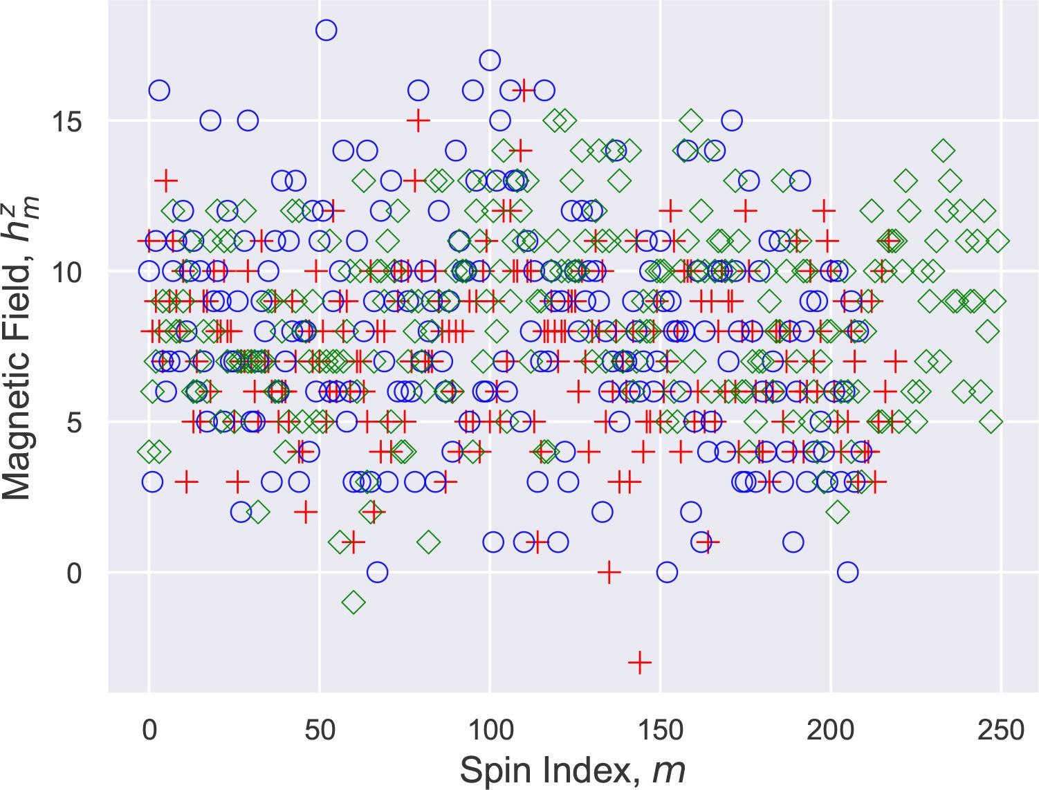
The spin representations of three Sudoku puzzles published in The New York Times on January 2 (diamond), January 12 (circle), and January 14 (plus), 2025, are shown. The mean and standard deviation of the magnetic field
However, the minimization problem involves more than just the fluctuating magnetic field; the spins also experience strong interactions. Figure 2 shows the Ising couplings between the spins in the January 12 Sudoku puzzle. Each spin is represented by a dot, arranged along an elliptical track for clearer visualization. A line connecting spins m and n ≠ m indicates a nonzero coupling Jm,n. It is clear that the interactions are long-ranged, extending beyond just nearest neighbors. Closer inspection reveals that there are a total of 1,261 connections among the Ns = 210 spins, and all couplings are of equal strength, with Jm,n = 2. A positive coupling constant J corresponds to antiferromagnetic interactions, which energetically favor opposing spin orientations. However, satisfying the competing preferences of all these couplings simultaneously is generally impossible, a phenomenon known as frustration [30]. These two factors—long-range interactions and frustration—greatly complicate the spin optimization problem.
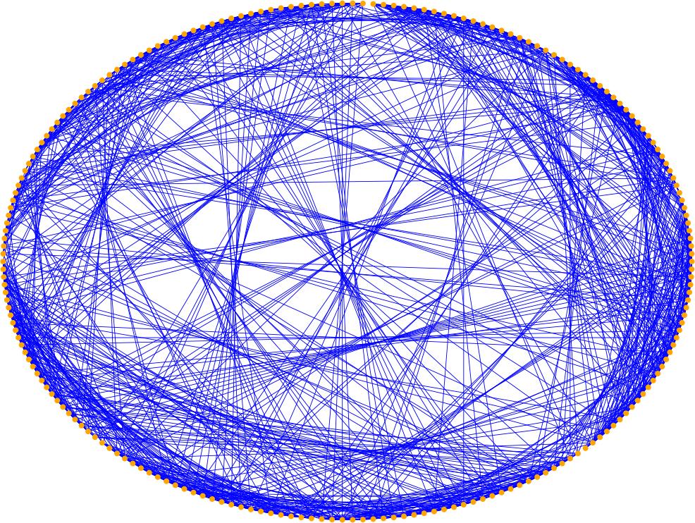
The dense, long-range couplings among the 210 spins for the January 12, 2025, Sudoku puzzle. Each line represents an Ising coupling Jm,n = 2, which favors spin-m and spin-n being antiparallel. Each spin can point either up or down. Finding the lowest-energy spin configuration corresponds to solving the Sudoku puzzle.
Since the long-range Ising interactions play a crucial role in our algorithm design, we separately count the number of nonzero Jm,n values as a function of the distance d = |m – n| between spins. The results are shown in Figure 3 for the same three puzzles presented in Figure 1. The vertical axis, plotted on a logarithmic scale, represents the filling fraction ρ(d), which is defined as the number of couplings between spins separated by distance d, divided by (Ns – d)—the maximum number of possible connections at distance d.
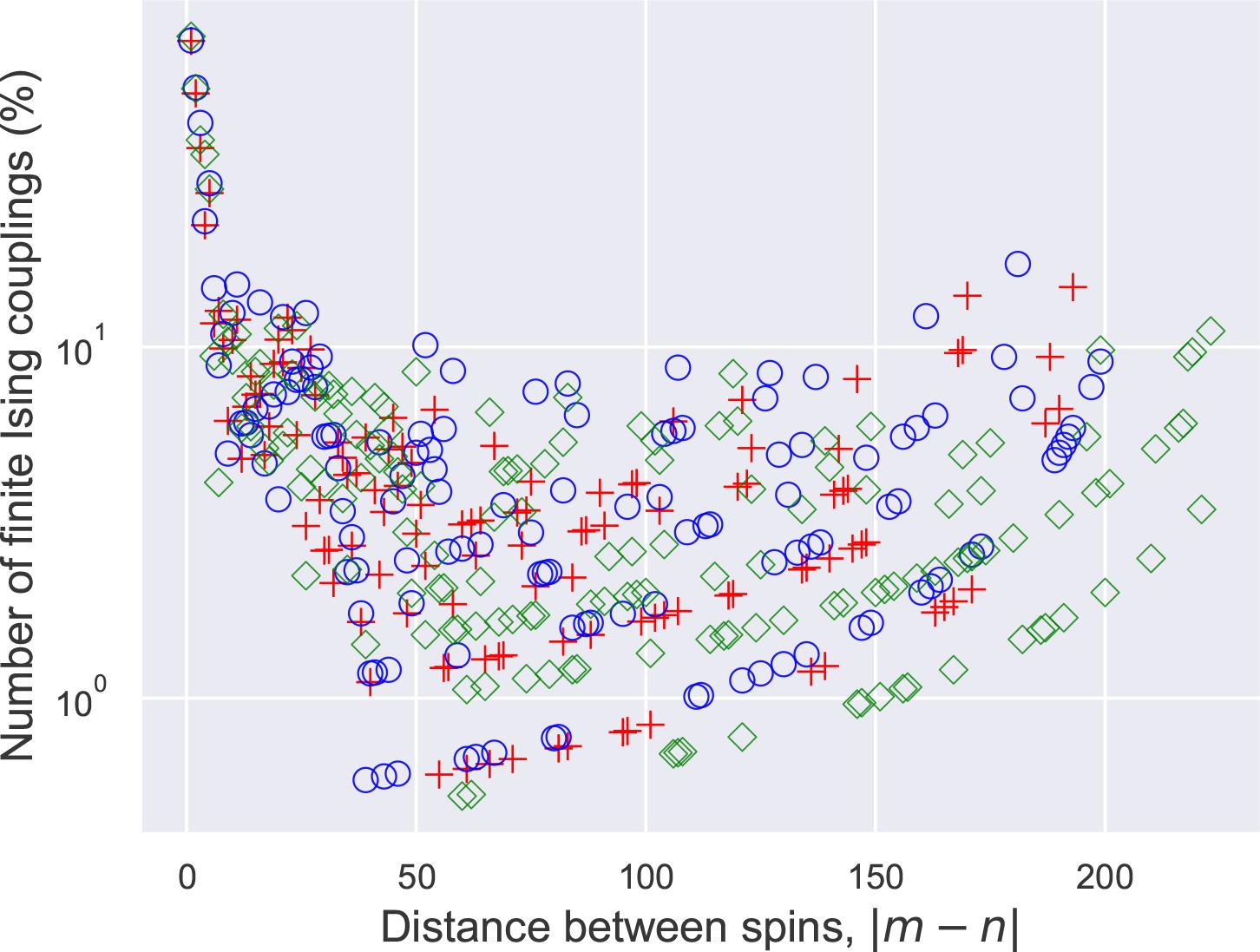
Statistical analysis of the couplings between the spins. For nearest neighbors, about 75% are coupled. The coupling fraction drops to the 10% level when the distance grows to 6 or 7, then fluctuates between 1% and 10%. The legends are the same as Figure 1. The vertical axis is in logarithmic scale.
We observe that nearest-neighbor couplings (d = 1) are present in approximately 75% of the possible cases. The filling fraction decreases sharply, dropping to around 10% by d = 6, and then fluctuates between 1% and 10% for larger distances. Interestingly, at long distances, ρ(d) begins to converge into a few smooth curves. This behavior can be traced back to the structure of the Sudoku grid and the uniform penalty terms used in the formulation.
Finally, we note that for the Sherrington-Kirkpatrick spin glass, the energy gap that separates the ground state from the first excited state is randomly generated and can be very small. This stands in contrast to the Sudoku problems where the gap is finite and known.
A popular heuristic approach for solving QUBO problems is quantum annealing [10–12], which utilizes specialized quantum hardware, such as D-Wave’s Advantage annealer [15]. The central idea is to engineer a time-dependent Hamiltonian, typically of the form:
In practice, several factors affect the efficacy of quantum annealing. First, during the time evolution, if the energy gap (the difference between the ground state and the first excited state) of H(s) becomes vanishingly small, the time τ required for quantum annealing may grow exponentially. For finite annealing schedules, the final state will no longer be the ground state of H1, and contributions from excited states could disrupt the QUBO solution. Second, a faithful implementation of H(s) requires full connectivity between the spins. For example, the dense connection pattern in Figure 2 differs from D-Wave’s Pegasus graph, where each qubit (spin) is only coupled to 15 other qubits in a periodic pattern [15]. Consequently, many QUBO problems must undergo a process called embedding to fit into the annealer’s hardware [15]. Third, quantum annealers often come with costs or restrictions on the running time, making them impractical for many users with limited resources.
These limitations motivate us to develop a quantum-inspired algorithm for solving QUBO problems. The term “quantum-inspired” is used in line with the review article [20], where it refers to algorithms that draw inspiration from quantum computation and information techniques but operate on classical data (e.g., from Sudoku or MaxCut problems) and run on classical computers rather than quantum hardware. Specifically, we map the classical problem in equation (16) to a quantum spin problem in equation (19) and simulate the quantum spin system classically using its tensor network representation. This approach is feasible because the low-energy quantum states of certain classes of spin Hamiltonians can be efficiently expressed as tensor networks, which can be manipulated within polynomial time [23]. We will show that the quantum-inspired algorithm proposed here, sitting between classical methods such as simulated annealing and quantum hardware-based algorithms like quantum annealing and QAOA, can circumvent some of the drawbacks associated with quantum annealing.
A key component of our quantum-inspired algorithm is the tensor network representation of many-spin wave functions [23,26]. In particular, we leverage the Matrix Product States (MPS) formalism to efficiently represent and manipulate quantum spin states on classical computers. Existing tensor network approaches to QUBO problems— such as those recently proposed by Patra et al. [31] and Mugel et al. [21]—typically aim to find ground states of Ising spin glass models via imaginary-time evolution. However, this method can be computationally expensive, especially for systems with long-range interactions.
To address this challenge and better guide the MPS toward the ground state, we adopt an alternative approach based on the Density Matrix Renormalization Group (DMRG) [24,25]. DMRG is an iterative variational algorithm that optimizes MPS representations by “sweeping” through the spin chain multiple times to progressively minimize the system’s energy. A brief introduction to MPS and DMRG, along with relevant references, is provided in Appendix A.
In addition to MPS and DMRG, the third ingredient of our algorithm is the driver Hamiltonian, a concept borrowed from quantum annealing (analogous to the mixer Hamiltonian in QAOA). Instead of using the traditional, slow, continuous annealing schedule s(t) employed in quantum annealing, we adopt a discrete M-step driving schedule to steer the system toward the ground state.
The Hamiltonian at the i-th step is given by
The algorithm proceeds as described in Algorithm 1.
1: Choose an initial matrix product state |ψ0〉.
2: for i = 1 to M do
3: update the MPS for Hi from |ψi–1 〉 to |ψi〉 by DMRG sweeps,
4: end for
5: return |ψM 〉
Once we obtain |ψM〉 from Algorithm 1, the ground state of the Ising spin glass Hz, we can compute both the ground energy EM and the corresponding spin configuration. We shall show in Section 4 and Section 5 below that the combination of MPS, DMRG and discrete driving provides a more tractable and efficient approach for QUBO problems.
One might wonder why we don’t simply use DMRG to find the ground state of Hz directly, thereby bypassing all the preceding steps up to i = M – 1. The reason is that DMRG rarely works effectively without a good initial guess for the starting state. While DMRG is an excellent tool for finding the ground state of one-dimensional gapped Hamiltonians with local interactions, it can easily get stuck in local minima when applied to glassy or long-range Hamiltonians, such as Hz. In our algorithm, all the preceding steps are designed to create a pathway that successively steers the MPS state:
Our algorithm is implemented in Julia 1.10.5, using the ITensors library version 0.6.23 to carry out the MPS and DMRG calculations [32]. All runtime data were collected on a laptop equipped with an Apple M3 chip.
The discrete driving schedule proposed here bears some resemblance to the concept of “fictitious time” used in quantum annealing via path-integral Monte Carlo [33,34], where a transverse field is decreased over a series of discrete Monte Carlo steps. However, it is important to note that the number of Monte Carlo steps in such methods is typically very large (up to 106) [33], whereas the number of driving steps employed in our work is comparatively small—on the order of 10.
In this section, we test the performance of our algorithm by applying it to solve the Sudoku puzzles published daily by The New York Times [35]. This choice is inspired by an example presented by Mücke [22]. A key advantage of using these puzzles is that they are archived and readily accessible online [36].
Table 1 presents a few examples. Each row lists a puzzle, uniquely identified by its date of publication and assigned difficulty level, where “m” stands for intermediate and “h” for hard. Also displayed for each puzzle are the number of clues (Nc), the number of up spins in the correct solution (N↑), the total number of spins (Ns) in the corresponding Ising spin glass Hz, and the constant energy shift c1 + c2 + c3 in Hz (see (16)). A successful run of the algorithm should drive the energy down to zero. For verification, we take the converged spin configuration, translate it back to the X variables, then to the full QUBO vector Z, and print the completed Sudoku board to ensure that all numbers fit correctly and none of the constraints are violated.
A few examples of solved Sudoku puzzles in chronological order according to their publication date in The New York Times. These puzzles vary in the number of clues (Nc), total number of spins (Ns), and other parameters; see the main text for details.
| Puzzle date | Level | Nc | N↑ | Ns | c1+c2+c3 |
|---|---|---|---|---|---|
| January 8, 2024 | h | 24 | 57 | 211 | 368.5 |
| December 10, 2024 | m | 26 | 55 | 200 | 359.0 |
| January 2, 2025 | m | 22 | 59 | 250 | 520.5 |
| January 8, 2025 | m | 23 | 58 | 232 | 461.5 |
| January 12, 2025 | m | 27 | 54 | 210 | 426.5 |
| January 14, 2025 | m | 23 | 58 | 232 | 457.0 |
| January 15, 2025 | m | 25 | 56 | 210 | 380.0 |
We discuss a few examples in some detail to illustrate how the algorithm parameters are chosen for the calculations. For the January 8, 2024, puzzle, listed in the first row of the table, we start from the state (21), which is an equal-weight superposition of all Sz basis states, and use a homogeneous transverse field
For DMRG, we set the maximum bond dimension D = 60 and perform 5 sweeps at each stop i. With these settings, the proposed algorithm successfully solves the puzzle. Both Hi and |ψi⟩ change with i, so the time spent on each DMRG sweep varies roughly from 0.1 to 8 seconds. In fact, the algorithm spends most of its time on Hi<M to steer the MPS. During these steps, the MPS have D = 60, which makes them computationally expensive. Only in the last step (i = M) is the problem Hamiltonian Hz considered. This final stage is efficient and fast: the MPS typically converges within 3 DMRG sweeps, and the bond dimension drops from 60 to 1, meaning the ground state becomes a product state, as expected. The quick convergence is largely due to the proximity of |ΨM–1⟩ from the preceding steps to the true ground state |ψM⟩.
Both the initial state and the driving schedule used here resemble those in quantum annealing. This is intentional, allowing us to take advantage of superposed states and the mixer Hamiltonian. However, the similarity ends there. Our algorithm does not follow any adiabatic time evolution, so the “trajectory” of the MPS wave function from |ψ0⟩ to |ΨM is fundamentally different. The algorithm is largely insensitive to the choice of |ψ0⟩, as long as it serves as a reasonable starting point for the DMRG solution of H1, which is predominantly Hx with only a small admixture of Hz.
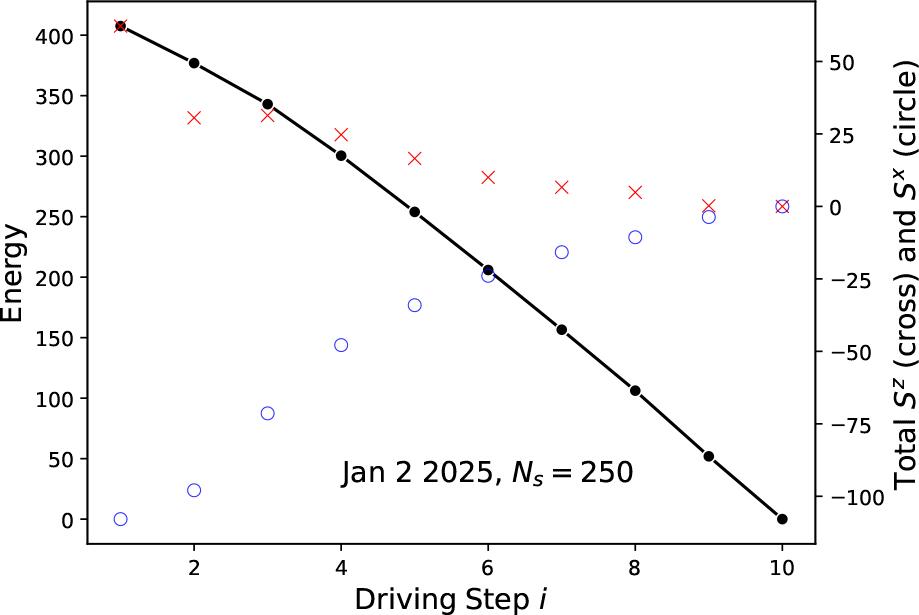
To demonstrate the flexibility of the algorithm, we use the same puzzle but start from a random MPS with bond dimension 3 and choose D = 20 for all subsequent steps. The puzzle is solved successfully at a much faster pace, with each sweep taking about 0.8 seconds. As shown in Figure 4, the energy (black dots) steadily drops to zero. To track the spins’ behavior at each step, we define the total spin-z operator measured from its ground state value
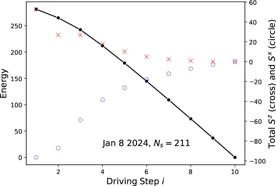
How the January 8, 2024, puzzle gets solved: As the driving field hx is reduced, the energy gradually drops to zero. The total spin along the x-direction vanishes, while the total spin along the z-direction approaches its ground state value. The bond dimension is D = 20, and the driving field is set to hx = 0.75.
The red crosses in Figure 4 show the expectation values of Sz (magnified by a factor of 4 to be clearly visible). Figure 4 also includes the expectation values (blue circles) of the total spin-x operator defined by
As the weight of Hx is decreased and the weight of Hz is increased during the driving process, Sx gradually approaches zero, while Sz converges to its ground state value
If the primary concern is the wall time for solving the 9 × 9 Sudoku puzzles, our algorithm pales in comparison to classical algorithms that build on logic and exploit the structure of the problem. In contrast, the QUBO approach to Sudoku puzzles, as noted earlier, is not efficient and resembles more of a blind search. The problem is treated simply as another QUBO matrix, and the solution strategy here does not focus on the underlying meaning of the original constraints. However, this apparent weakness can be turned into a strength. As the board size increases, the algorithm is expected to outperform conventional methods since the calculation scales as NsD3M. More importantly, it can be applied to other QUBO problems, as we will demonstrate in Section 5.
Other puzzles listed in the table are solved in a similar manner. Since they differ in Ns,
Within the table, the January 2, 2025, puzzle has the least number of clues and the maximum number of spins, Ns = 251. The broad features of its solution process can be appreciated from Figure 5, which is comparable to our earlier example in Figure 4. In both cases, the energy decreases with i, but not exactly in a linear fashion. To quantify this, let Ei be the energy achieved at the ith driving step. If we draw a straight line from the starting point (i = 1, E1) to the ending point (i = M, EM), then let δEi be the deviation of Ei from this line. We plot δEi in Figure 6 for a few solved puzzles. The energy drop is clearly sub-linear, and the peak location of δEi correlates with the inflection point of the total Sx. A more detailed picture of the solution process is provided in Figure 7. Here, the horizontal axis represents the spin index m = 1 to 251, going from left to right. The vertical axis corresponds to the driving step i = 1 to M = 10, going from top to bottom. On each row, shown in false color, are the expectation values of the spin-z operator,
The solution process for another puzzle with fewer clues and more spins: D = 20, hx = 1.
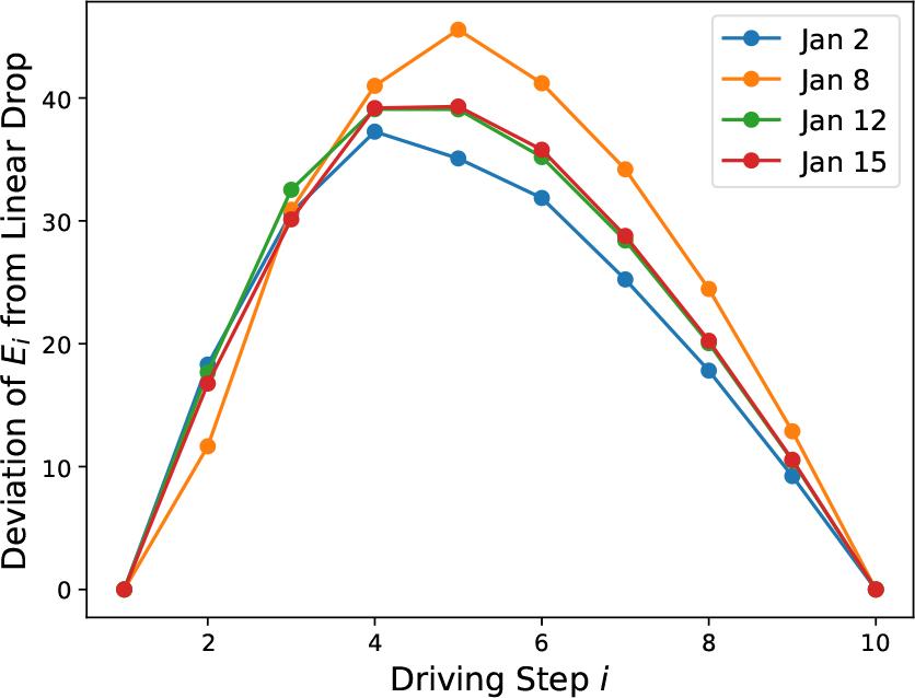
The nonlinear drop in energy during the driving process. See main text for details.
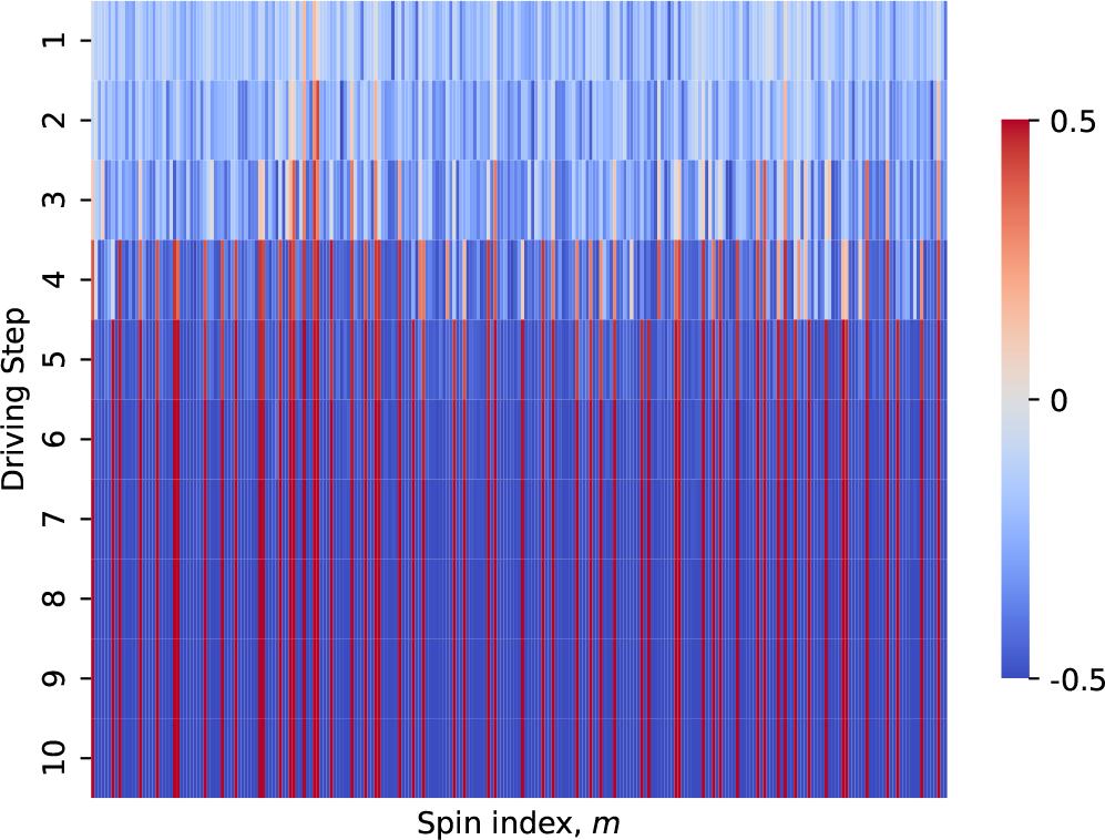
The evolution of the 251 spins during the solution process of the January 2, 2025, puzzle. The value of
We observe that in the initial steps, due to the hx field,
| 2 | 8 | 1 | 3 | 5 | 4 | 6 | 7 | 9 |
| 9 | 7 | 3 | 8 | 1 | 6 | 5 | 2 | 4 |
| 5 | 6 | 4 | 7 | 9 | 2 | 8 | 1 | 3 |
| 1 | 3 | 9 | 4 | 6 | 8 | 2 | 5 | 7 |
| 8 | 2 | 5 | 9 | 7 | 3 | 1 | 4 | 6 |
| 6 | 4 | 7 | 5 | 2 | 1 | 9 | 3 | 8 |
| 4 | 9 | 2 | 6 | 3 | 5 | 7 | 8 | 1 |
| 3 | 5 | 6 | 1 | 8 | 7 | 4 | 9 | 2 |
| 7 | 1 | 8 | 2 | 4 | 9 | 3 | 6 | 5 |
Interestingly, this valid solution differs from the one offered in [36]. Our quantum-inspired algorithm has found an independent solution!
We conclude the case study of Sudoku with a final remark. Our algorithm is heuristic and relies on several tuning parameters. It is unrealistic to expect a universal set of fail-safe parameters that can solve all Sudoku puzzles, as they translate into very different spin Hamiltonians. Therefore, some trial and error may be required when tackling a new puzzle. Compared to hardware-based quantum algorithms, a major advantage of our quantum-inspired approach is the explicit knowledge of the MPS wave functions, which allow for a detailed diagnosis of the solution process. As demonstrated above, in Figures 4 through 7, this analysis helps us fine-tune the initial state, driver, driving schedule, and other parameters. These strategies for parameter optimization will be further discussed when the algorithm is applied to MaxCut problems.
In this section, we apply the proposed algorithm to MaxCut, one of the most well-known problems in combinatorial optimization [37]. The goals are twofold: First, by testing it on new problem instances, we demonstrate the versatility of the algorithm and its capability to solve QUBO problems with varying characteristics. Second, by analyzing its performance across different problem sizes and types, we illustrate how the algorithm can be fine-tuned to optimize its performance for specific instances.
The MaxCut problem is defined on an undirected graph G = (V, E), where V represents a set of vertices and E represents a set of edges. An edge connecting vertex i and vertex j is denoted by (i, j) ∈ E and is assigned a weight wi,j. The objective is to partition V into two sets, V = A ∪ Ā with A ⋂ Ā = ∅, such that the weighted sum of the edges connecting A to Ā is maximized. This problem is NP-hard, and its connection to spin glass Hamiltonians has long been recognized [37,38].
To cast the problem into QUBO form, let us define the binary variable xi = 1 if vertex i belongs to set A, and xi = 0 otherwise. The edge (i, j) is part of the cut if and only if xi ≠ xj, i.e., (xi – xj)2 = 1. Therefore, the objective is to maximize the cut value.
It is easy to cast f into the standard QUBO form
We evaluate the performance of the algorithm using MaxCut instances drawn from the Biq Mac Library. All instances used in this section are available for download at [39] or alternatively at [40]. We will refer to each instance by its file name, which contains NV, the number of vertices. Note that the complexity of the problem also depends crucially on NE, the number of edges, as well as the values of wi,j. In what follows, we discuss three batches of test cases, labeled (I) to (III), with increasing difficulty. Each batch has a distinctive distribution of edge weights.
Twenty weighted MaxCut instances and the parameters used to solve them. Each instance is identified by its file name in the Biq Mac Library. The edge weights are either 1 or – 1. For the first ten instances, the number of vertices NV = 80 and the number of edges NE = 316. For the next ten instances, NV = 100 and NE = 495. The algorithm successfully finds E0, the ground state energy of the spin model (the MaxCut value is simply – E0), except for the case pm1s_100.5.
| Instance | E0 | M | hx | η | D |
|---|---|---|---|---|---|
| pm1s_80.0 | –79 | 5 | 1 | 0 | 30 |
| pm1s_80.1 | –69 | 5 | 1 | 0 | 30 |
| pm1s_80.2 | –67 | 5 | 1 | 0.3 | 30 |
| pm1s_80.3 | –66 | 5 | 1 | 0 | 30 |
| pm1s_80.4 | –69 | 5 | 1 | 0.3 | 30 |
| pm1s_80.5 | –66 | 20 | 1 | 0.3 | 30 |
| pm1s_80.6 | –71 | 5 | 1 | 0 | 30 |
| pm1s_80.7 | –69 | 5 | 1 | 0 | 30 |
| pm1s_80.8 | –68 | 5 | 1 | 0 | 30 |
| pm1s_80.9 | –67 | 5 | 1 | 0 | 30 |
| pm1s_100.0 | –127 | 5 | 1 | 0.3 | 30 |
| pm1s_100.1 | –126 | 5 | 1 | 0.3 | 30 |
| pm1s_100.2 | –125 | 10 | 1 | 0.3 | 30 |
| pm1s_100.3 | –111 | 10 | 1 | 0.3 | 30 |
| pm1s_100.4 | –128 | 5 | 1 | 0.3 | 30 |
| pm1s_100.5 | – | 10 | 1 | 0 | 60 |
| pm1s_100.6 | –122 | 10 | 1 | 0.3 | 30 |
| pm1s_100.7 | –112 | 20 | 1 | 0.3 | 60 |
| pm1s_100.8 | –120 | 10 | 1 | 0.3 | 30 |
| pm1s_100.9 | –127 | 5 | 1 | 0.3 | 30 |
These are weighted MaxCut problems where the edge weight wi,j is set to either 1 or – 1. An example is illustrated in Figure 8(a), which features 100 nodes and 495 edges. The edges are color-coded: green for wi,j = 1 and blue for wi,j = – 1. It is helpful to compare Figure 8 with the Sudoku example in Figure 2, where the edge weight is constant. In the MaxCut case, the edges are not only denser but also carry signs. In the spin language, this means there are more couplings among the Ising spins, and the coupling can be either ferromagnetic or antiferromagnetic. Also, the magnetic field along the z-axis for each spin m vanishes in this case, i.e.,
Despite these differences, our algorithm successfully solves all instances listed in Table 2, yielding the correct MaxCut values, with one exception: the instance named pm1s_100.5. In this case, the lowest energy obtained, E0 = –125, is above the value of –128 quoted in [39,40]. To alert the reader, the E0 value is underscored to indicate that this case remains unresolved. The parameters used in each instance (number of driving steps M, transverse field hx and its random fluctuations η, and bond dimension D) are listed in Table 2. Five DMRG sweeps are used for each driving step, with one exception: for pm1s_100.6, 10 sweeps are used to improve accuracy.
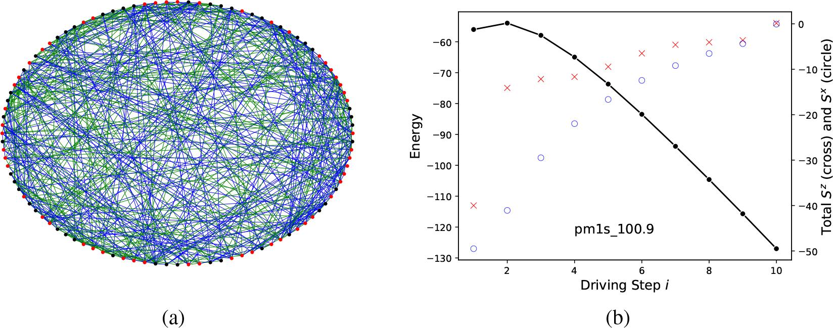
(a) Graph representation of the problem. The edges carry weights of 1 (in green) or – 1 (in blue). The solution is indicated by the node color: nodes in black belong to set A, while the rest of the nodes (in red) belong to set Ā. (b) The energy (dot), expectation values of Sz (cross, measured from its ground state value and magnified by 10 times), and Sx (circle) during the driving process. Solving the weighted MaxCut instance pm1s_100.9 from the Biq Mac Library.
Note that the algorithm parameters listed in the tables in this section may not be optimal. The problem can sometimes be solved with fewer resources than listed here.
Comparing the rows of Table 2 reveals some strategies for solving new QUBO problems. Within each group of MaxCut instances of similar size, some instances (e.g., pm1s_80.5 and pm1s_100.7) are more challenging to optimize. It is also generally harder to reach the ground state for instances with larger NV and NE. To tackle these harder cases, increasing the driving steps M and shaking the system with random fluctuations η often helps. Sometimes, increasing the bond dimension (e.g., D = 60 for pm1s_100.7) is necessary. Typically, these tuning decisions are made by monitoring the convergence of energy during the driving process. One example is shown in Figure 8(b) for the instance pm1s_100.9.
Twenty unweighted MaxCut instances from the Biq Mac Library with dense edges. The first ten cases have NV = 60 and NE = 885, while the remaining cases have NV = 100 and NE = 2,475. All edge weights are set to 1. The algorithm successfully solves all instances except g05_100.3 and g05_100.5, where the E0 values should be – 1,424 and – 1,436, respectively [39,40]. Here, Nsw refers to the number of DMRG sweeps per driving step, with hx = 1 and η = 0.3.
| Instance | E0 | M | Nsw | D |
|---|---|---|---|---|
| g05_60.0 | –536 | 10 | 5 | 30 |
| g05_60.1 | –532 | 10 | 5 | 40 |
| g05_60.2 | –529 | 10 | 5 | 30 |
| g05_60.3 | –538 | 10 | 5 | 30 |
| g05_60.4 | –527 | 10 | 5 | 30 |
| g05_60.5 | –533 | 10 | 5 | 30 |
| g05_60.6 | –531 | 10 | 5 | 30 |
| g05_60.7 | –535 | 10 | 5 | 60 |
| g05_60.8 | –530 | 10 | 5 | 30 |
| g05_60.9 | –533 | 20 | 5 | 40 |
| g05_100.0 | –1430 | 20 | 5 | 40 |
| g05_100.1 | –1425 | 20 | 5 | 40 |
| g05_100.2 | –1432 | 20 | 5 | 40 |
| g05_100.3 | –1423 | 10 | 5 | 30 |
| g05_100.4 | –1440 | 20 | 5 | 40 |
| g05_100.5 | –1435 | 10 | 5 | 30 |
| g05_100.6 | –1434 | 10 | 10 | 40 |
| g05_100.7 | –1431 | 10 | 10 | 40 |
| g05_100.8 | –1432 | 10 | 10 | 60 |
| g05 100.9 | –1430 | 10 | 10 | 40 |
These are unweighted MaxCut problems where all the edges share the same weight of 1, but the connections are much denser than in the first batch. For instance, the problem shown in Figure 9(a) has the same number of nodes as in Figure 8, but the number of edges has increased fivefold to 2475. The spin-spin coupling is so dense that it may seem challenging for MPS and DMRG, as they are typically known to work well with spin Hamiltonians involving local interactions. Amazingly, the algorithm continues to yield correct MaxCut values with only a moderate increase in the bond dimension D, despite the steep rise in NE.
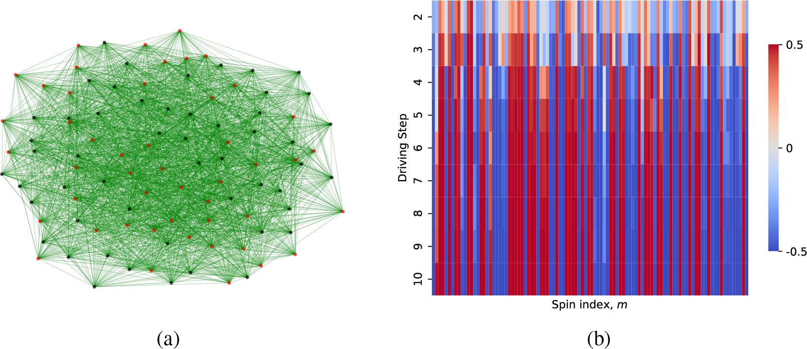
(a) Graph representation of the problem. All edges (green lines) carry equal weight of 1. The MaxCut found by our algorithm is color-coded: nodes in black belong to set Ā, while nodes in red belong to set Ā. (b) The expectation value of
The heatmap of
Note that there are two cases in Table 3 (with the E0 values underscored) where the algorithm came very close to the ground state but did not quite reach it.
The algorithm parameters used to successfully solve five MaxCut instances from the Biq Mac Library with 251 vertices and over 3200 edges, each with integer weights; D = 30, M = 10.
| Instance | E0 | NV | NE | hx | η | Nsw |
|---|---|---|---|---|---|---|
| bqp250-2 | -44810 | 251 | 3285 | 0.05 | 0 | 10 |
| bqp250-4 | -41274 | 251 | 3397 | 0.05 | 0 | 10 |
| bqp250-6 | -41014 | 251 | 3433 | 0.30 | 0 | 5 |
| bqp250-8 | -35726 | 251 | 3265 | 0.05 | 0 | 10 |
| bqp250-10 | -40442 | 251 | 3294 | 1.00 | 0.3 | 5 |
The third batch of instances includes even larger MaxCut problems with NV = 251 and NE exceeding 3200. The coupling between the nodes is so dense that these instances are not easily graphed or visualized. More importantly, in contrast to the examples discussed earlier, the edge weights in these instances vary over a wide range. For instance, the edge weight distribution of the instance bqp250-10 is shown in Figure 10. While there are a few outliers, the majority of wi,j fall within the range from –100 to 100, regardless of |i – j|, the distance between nodes. Other instances listed in Table 4 follow a similar distribution for wi,j. As a result, the numerical scale of the QUBO matrix and the energy scale of the spin-spin interaction differ significantly from previous examples. To make the algorithm less sensitive to the overall numerical scale of wi,j, we rescale the problem by dividing the matrix wi,j by the maximum absolute value of its elements. After this, |wi,j| becomes typically much smaller than 1. Consequently, the value of hx is smaller compared to previous examples, as shown in the fifth column of Table 4.
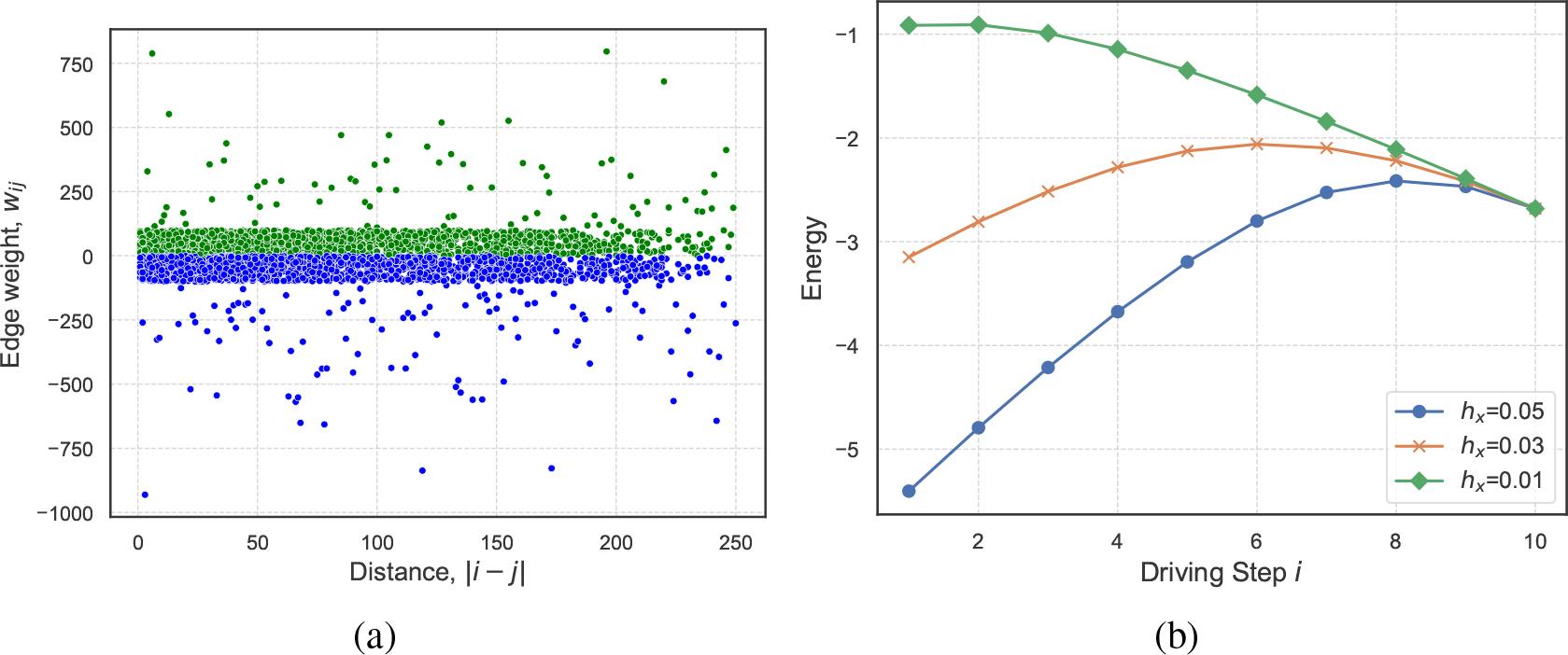
(a) The distribution of the edge weights wi,j sorted by |i – j|, the distance between the nodes. Most of the weights lie within the interval from –100 to 100. (b) The variation of energy during the driving process for three different values of hx. All three choices converge to the ground state, yielding the correct MaxCut value. The edge matrix has been normalized such that the maximum absolute value of its elements is 1. Solving MaxCut instance bqp250-8 with 251 nodes and 3265 edges.
It’s important to note that the choice of hx is not unique. Figure 10(b) compares the energy for three different values of hx during the driving process. All three configurations lead to the correct ground state, demonstrating the robustness of the algorithm, even with the significant increase in NE and NV.
To summarize this section, we find it encouraging that the proposed quantum-inspired algorithm is capable of solving a wide variety of MaxCut problems of different sizes and types. However, success is not always guaranteed. Some cases prove to be more stubborn, resisting energy minimization. This is not unexpected, as similar challenges are frequently encountered in quantum annealing, where techniques like reverse and cyclic annealing have been introduced to prevent the system from becoming trapped in local minima. Refining and enhancing our algorithm to address such challenges will be part of future work.
It is important to note that all QUBO problems can be formulated as MaxCut problems. Indeed, all the instances in Table 4 were originally generated as QUBO problems by Beasley [41] and later translated into MaxCut format. Thus, the key takeaway from this section is that the quantum-inspired algorithm based on MPS and DMRG is versatile and continues to perform effectively on MaxCut (and, more broadly, QUBO) problems of larger sizes with denser connections.
The emerging field of solving combinatorial optimization problems using quantum-inspired algorithms based on tensor networks is still in its early stages. Previous works have focused on the imaginary time evolution of MPS and experimented with PEPS [21,31], where the main approach was to solve the problem Hamiltonian directly. Our algorithm, presented in Section 3, differs in two significant ways. First, we introduce a driver/mixer Hamiltonian and work with a discrete driving schedule. Second, at each driving stage, we use DMRG to update the MPS wave function, progressively steering it toward the ground state of the problem Hamiltonian. In Sections 4 and 5, we presented conclusive evidence that the algorithm can successfully solve a variety of Sudoku puzzles and MaxCut problems. To our knowledge, the combination of DMRG with discrete driving has not been demonstrated before in the context of QUBO problems, and the application of DMRG to Ising spin glass Hamiltonians with long-range interactions has not been systematically analyzed.
The algorithm proposed here is general and can be adapted to a wide range of QUBO problems. The problem sizes presented in Sections 4 and 5 (up to 251 spins with 3,265 couplings, which exceeds the capabilities of state-of-the-art QAOA) are kept relatively small, allowing most calculations to be completed on a laptop within a few minutes to an hour. The main goal of this work is to establish the feasibility of the proposed algorithm and test it across problems of diverse origin and size, while ensuring that the iterations remain fast and computationally inexpensive. In future work, we plan to explore how the algorithm can scale to tackle practical large-scale problems. For example, a popular choice for benchmarking many state-of-the-art MaxCut solvers is Gset, which includes problems with over 800 (up to 20,000) vertices [42]. For such large problems, different trials with varied initial MPS or driving parameters could be run in parallel on high-performance computing clusters over days or weeks.
Tensor network analysis of glassy spin Hamiltonians also provides new insights into algorithm design. Quantum annealing is inherently heuristic, and when faced with a new problem Hamiltonian, it is not immediately clear which driver Hamiltonian and annealing schedule will offer the best chance of reaching the global minimum. Without a precise understanding of the dynamics of interacting spins (qubits), the annealing process could result in either a success or failure. The many-spin wave functions obtained from tensor network calculations offer detailed information about the system under driving. This diagnostic data translates into a deeper understanding of the role of each parameter, aiding in more informed decisions when selecting algorithmic parameters. The ability to directly access the quantum states is a significant strength of the quantum-inspired approach.
Quantum optimization algorithms, such as quantum annealing and QAOA, hold great potential to surpass classical algorithms for industrial-scale optimization problems. In the near term, however, their performance will be limited by the capabilities of current hardware. Before these quantum algorithms can reach their full potential, quantum-inspired algorithms can bridge the gap by solving middle-to large-scale problems within polynomial time via quantum simulations on classical computers. A few recent examples, some of which are not directly related to optimization tasks, illustrate the potential of tensor network calculations. IBM’s 127-qubit Eagle processor initially showed experimental results on two-dimensional quantum spin systems that were believed to have achieved quantum advantage—i.e., performing “accurate computations at a scale beyond brute-force classical simulation” [43]. However, soon after, improved tensor network calculations on classical computers produced more accurate results than the quantum processor [44]. Tensor networks have also been used to replace parts of the QAOA [45] or quantum annealing [46] algorithms. In yet another recent development, several quantum-inspired solvers based on tensor trains were demonstrated to successfully solve nonlinear partial differential equations [47–50]. These examples further underscore that tensor network methods are powerful and versatile tools, extending beyond combinatorial optimization problems. The near-term landscape of optimization will likely feature a coexistence where quantum-inspired algorithms and pure quantum algorithms compete and complement each other.