
Table 1.
Our best-performing 8th order solutions when setting m = 10.
| Best 8th order for spectral-norm error | Best 8th order for eigenvalue error | |
|---|---|---|
| w1 | 0.59358060400850625863514059265224 | 0.10467636532245895252340732579853 |
| w2 | −0.46916012347004197296293264921328 | −0.57896999331780988041471955125778 |
| w3 | 0.2743566425898467907228242878146 | 0.57503350160061785946141563279891 |
| w4 | 0.17193879484656773059919074965377 | 0.12231011868707029786561397542663 |
| w5 | 0.23439874482541384415430578747541 | 0.27793149999039524816733903301747 |
| w6 | −0.48616424480326193899617759997914 | −0.37349605088056728482635987352576 |
| w7 | 0.49617367388114660354871757044906 | 0.11575566589480463220616543972403 |
| w8 | −0.32660218948439130114501815323814 | 0.1464645610975800618712569230326 |
| w9 | 0.23271679349369857679445410270557 | −0.39443578322284085764474498594073 |
| w10 | 0.098249557414708533273471906180643 | 0.44370228726021218923197141183196 |
Table 2.
Our best-performing 8th order kernel and processor when setting m = 8. The value of γ10 for the processor is chosen such that the sum is zero.
| Best 8th order kernel | Processor for kernel | ||
|---|---|---|---|
| w1 | 0.21784176681731006074681969186513 | −0.44324901019570126590495430949294 | γ1 |
| w2 | 0.1947017706053903224022456342907 | 0.25459857192003772850622377066944 | γ2 |
| w3 | 0.18372413281145589944261642180363 | −0.73862036266779261573694538099739 | γ3 |
| w4 | −0.37307499512657736825709230652023 | −0.00024139614958652134370419495289618 | γ4 |
| w5 | 0.15757644257569146373033662060461 | 0.73873460354125365739379753874964 | γ5 |
| w6 | −0.33342207567391682979227850551172 | −0.20285971152536085519251666906017 | γ6 |
| w7 | 0.51788649682987924281787142226803 | 0.44989521689676869571827637424046 | γ7 |
| w8 | 0.21456475499897766986381219621761 | 0.29538398007876871184026747505657 | γ8 |
| −0.3364996155865700091428329802017 | γ9 |
Table 3.
The 10th order solution with lowest eigenvalue error in our numerical search.
| 10th order solution with m = 17 | |
|---|---|
| w1 | −0.28371232689144296279654621726493 |
| w2 | 0.046779504778147381605331000278223 |
| w3 | 0.36845892382797770619657504217539 |
| w4 | 0.19186204094674514739760408197461 |
| w5 | −0.53123134392680669702873064192428 |
| w6 | −0.0081253242720827266680816105600661 |
| w7 | −0.16389450414378567860032917538393 |
| w8 | 0.18514766119291405032528647881 |
| w9 | 0.5383584694754681989174668806505 |
| w10 | −0.30583981835573485697292316732177 |
| w11 | 0.43199935609523301289295473774488 |
| w12 | 0.1510502301631786853020124612813 |
| w13 | −0.35051099204829676098801520498121 |
| w14 | 0.1032971125844291674511513007661 |
| w15 | 0.15043936943817152697371946806229 |
| w16 | 0.12118469498650736511410491586846 |
| w17 | 0.10437742779547826358296681557444 |
Table 4.
The list of 4th order product formulae. The column labelled “processing” indicates whether the formula uses processor. The label is the name we will refer to the formula by. The constant factor in the error is denoted χ for spectral-norm error and ζ for eigenvalue error, and the corresponding quantities Mχ1/k and Mζ1/k are given. The column labelled S2 indicates whether the product formula is a product of S2. The best result is highlighted in green, and is from 2002 [47]. The 2006 result PPBCM4m6 is slightly higher error, but it is not evident to 2 significant figures.
| label | M | S2 | processing | reference | χ | Mχ1/k | ζ | Mζ1/k |
|---|---|---|---|---|---|---|---|---|
| S4m1 | 3 | Y | N | first fractal product [2] | 4.9 × 10⁻² | 1.41 | 2.3 × 10⁻² | 1.17 |
| S4m2 | 5 | Y | N | second fractal product [4] | 3.0 × 10⁻³ | 1.17 | 3.3 × 10⁻⁴ | 0.67 |
| O4M5 | 5 | N | N | Ostmeyer Eq. (40) of [46] | 3.0 × 10⁻⁴ | 0.66 | 7.7 × 10⁻⁵ | 0.47 |
| BM4M6 | 6 | N | N | S6 Table 2 of [47] | 1.6 × 10⁻⁴ | 0.67 | 2.4 × 10⁻⁵ | 0.42 |
| PPBCM4m6 | 6 | N | Y | P64 Table 5 of [31] | 5.7 × 10⁻⁵ | 0.52 | 2.4 × 10⁻⁵ | 0.42 |
| BCE4m3 | 6 | Y | Y | Table 6 of [40] | 1.6 × 10⁻² | 2.15 | 1.5 × 10⁻³ | 1.17 |
| BCE4m4 | 8 | Y | Y | Table 6 of [40] | 3.4 × 10⁻⁴ | 1.09 | 9.8 × 10⁻⁵ | 0.80 |
| BCE4m5 | 10 | Y | Y | Table 6 of [40] | 6.7 × 10⁻⁵ | 0.90 | 2.1 × 10⁻⁵ | 0.68 |
| BCE4m6 | 12 | Y | Y | Table 6 of [40] | 2.6 × 10⁻⁵ | 0.85 | 7.0 × 10⁻⁶ | 0.62 |
| BCE4m7 | 14 | Y | Y | Table 6 of [40] | 1.3 × 10⁻⁵ | 0.85 | 3.0 × 10⁻⁶ | 0.58 |
| BCE4m8 | 16 | Y | Y | Table 6 of [40] | 7.9 × 10⁻⁵ | 0.85 | 1.5 × 10⁻⁶ | 0.56 |
| BCE4m9 | 18 | Y | Y | Table 6 of [40] | 5.3 × 10⁻⁶ | 0.86 | 8.6 × 10⁻⁷ | 0.55 |
Table 5.
The list of 6th order product formulae with their average errors. The column labelled S2 indicates whether it is a product of S2. The best result is highlighted in green, and is from 2006 [31].
| label | M | S2 | processing | reference | χ | Mχ1/k | ζ | Mζ1/k |
|---|---|---|---|---|---|---|---|---|
| S6m1 | 9 | Y | N | first fractal product [2] | 4.5 × 10⁻² | 5.36 | 2.3 × 10⁻² | 4.81 |
| S6m2 | 25 | Y | N | second fractal product [4] | 1.3 × 10⁻⁵ | 3.83 | 2.0 × 10⁻⁷ | 1.91 |
| Y6m3a | 7 | Y | N | Solution A in Table 1 of [3] | 2.0 × 10⁻³ | 2.49 | 1.2 × 10⁻³ | 2.28 |
| KL6s9a | 9 | Y | N | s9odr6a in Appendix A of [25] | 2.9 × 10⁻⁴ | 2.31 | 1.7 × 10⁻⁴ | 2.12 |
| KL6s9b | 9 | Y | N | s9odr6b in Appendix A of [25] | 2.9 × 10⁻⁴ | 2.31 | 1.7 × 10⁻⁴ | 2.11 |
| SS6s11 | 11 | Y | N | Section 4.2 of [29] | 4.2 × 10⁻⁵ | 2.05 | 1.4 × 10⁻⁵ | 1.71 |
| SS6s13 | 13 | Y | N | Section 4.2 of [29] | 2.1 × 10⁻⁵ | 2.16 | 3.4 × 10⁻⁶ | 1.59 |
| BM6M10 | 10 | N | N | S10 Table 2 of [47] | 6.0 × 10⁻⁶ | 1.35 | 1.4 × 10⁻⁶ | 1.06 |
| PPBCM6m9 | 9 | N | Y | P96 Table 5 of [31] | 5.0 × 10⁻⁶ | 1.18 | 4.3 × 10⁻⁷ | 0.78 |
| PPBCM6m5 | 11 | Y | Y | P116 in Table 6 of [31] | 1.9 × 10⁻⁶ | 1.22 | 9.0 × 10⁻⁷ | 1.08 |
| PPBCM6m6 | 13 | Y | Y | P136 in Table 6 of [31] | 4.8 × 10⁻⁷ | 1.15 | 2.5 × 10⁻⁷ | 1.03 |
| BCE6m5 | 10 | Y | Y | Table 8 of [40] | 5.8 × 10⁻³ | 4.24 | 3.2 × 10⁻³ | 3.84 |
| BCE6m6 | 12 | Y | Y | Table 8 of [40] | 7.7 × 10⁻⁵ | 2.47 | 2.0 × 10⁻⁵ | 1.98 |
| BCE6m7 | 14 | Y | Y | Table 8 of [40] | 1.6 × 10⁻⁵ | 2.22 | 2.4 × 10⁻⁶ | 1.62 |
| BCE6m8 | 16 | Y | Y | Table 8 of [40] | 4.6 × 10⁻⁶ | 2.06 | 3.2 × 10⁻⁷ | 1.32 |
| BCE6m9 | 18 | Y | Y | Table 8 of [40] | 7.3 × 10⁻⁶ | 2.51 | 1.3 × 10⁻⁷ | 1.28 |
| BCE6m10 | 20 | Y | Y | Table 8 of [40] | 3.2 × 10⁻⁶ | 2.42 | 9.9 × 10⁻⁹ | 0.93 |
| BCE6m11 | 22 | Y | Y | Table 8 of [40] | 7.9 × 10⁻⁶ | 3.11 | 1.4 × 10⁻⁸ | 1.08 |
Table 6.
The list of 8th order product formulae with their average errors. This table shows our new results for product formulae that improve over those in the prior literature. The result that provides the most efficient simulations is highlighted in (dark) green, and is our processed product formula. That provides the best performance due to the shorter length, but the lowest error is provided by our product formula highlighted in (dark) blue. The lowest error results from prior work are highlighted in light blue (for the non-processed case), and light green (for the processed case). The processed product formula PP8s13 (P138) has larger error than the highlighted PP8s19, but better performance due to its shorter length.
| label | M | processing | reference | χ | Mχ1/k | ζ | Mζ1/k |
|---|---|---|---|---|---|---|---|
| S8m1 | 27 | N | first fractal product [2] | 5.6 × 10⁻² | 18.8 | 1.6 × 10⁻² | 16.2 |
| S8m2 | 125 | N | second fractal product [4] | 6.7 × 10⁻⁹ | 11.9 | 5.2 × 10⁻¹³ | 3.64 |
| Y8m7d | 15 | N | Solution D in Table 2 of [3] | 1.1 × 10⁻³ | 6.41 | 1.3 × 10⁻⁴ | 4.89 |
| MC8s15 | 15 | N | Table 2 of [24] | 6.5 × 10⁻⁶ | 3.37 | 2.0 × 10⁻⁶ | 2.90 |
| MC8s17 | 17 | N | Table 2 of [24] | 7.9 × 10⁻⁷ | 2.94 | 3.3 × 10⁻⁷ | 2.63 |
| KL8s17a | 17 | N | s17odr8a in [25] | 6.1 × 10⁻⁷ | 2.84 | 2.7 × 10⁻⁷ | 2.56 |
| KL8s17b | 17 | N | s17odr8b in [25] | 5.9 × 10⁻⁷ | 2.83 | 2.5 × 10⁻⁷ | 2.54 |
| SS8s19 | 19 | N | Section 4.3 of [29] | 1.8 × 10⁻⁷ | 2.72 | 5.3 × 10⁻⁸ | 2.34 |
| SS8s21 | 21 | N | Section 4.3 of [29] | 3.4 × 10⁻⁷ | 3.27 | 7.5 × 10⁻⁸ | 2.70 |
| PP8s13 | 13 | Y | P138 in Table 6 of [31] | 1.2 × 10⁻⁶ | 2.37 | 6.5 × 10⁻⁷ | 2.19 |
| PP8s19 | 19 | Y | P198 in Table 6 of [31] | NA | NA | 2.4 × 10⁻⁷ | 2.83 |
| Y8m10 | 21 | N | Table 1 (our new result) | 5.8 × 10⁻⁸ | 2.61 | 7.0 × 10⁻⁹ | 2.01 |
| Y8m10b | 21 | N | Table 1 (our new result) | 6.3 × 10⁻⁷ | 3.53 | 5.4 × 10⁻¹⁰ | 1.46 |
| YP8m8 | 17 | Y | Table 2 (our new result) | 5.3 × 10⁻⁸ | 2.09 | 8.1 × 10⁻¹⁰ | 1.24 |
Table 7.
The list of 10th order product formulae with their average errors. The best result is highlighted in green, and is the product formula from 2005 [29]. That product formula provides exceptional performance for 10th order, being about 280 times better than all others from prior work, and half the error of our solution (bottom line).
| label | M | processing | reference | χ | Mχ1/k | ζ | Mζ1/k |
|---|---|---|---|---|---|---|---|
| S10m1 | 81 | N | first fractal product [2] | 9.0 × 10⁻² | 63.7 | 2.7 × 10⁻³ | 44.8 |
| S10m2 | 625 | N | second fractal product [4] | 4.1 × 10⁻¹³ | 36.0 | 6.1 × 10⁻¹⁹ | 9.44 |
| KL10s31a | 31 | N | s31odr10a in Appendix A of [25] | 8.7 × 10⁻⁶ | 9.67 | 5.8 × 10⁻⁶ | 9.28 |
| KL10s31b | 31 | N | s31odr10b in Appendix A of [25] | 8.4 × 10⁻⁵ | 12.1 | 4.1 × 10⁻⁵ | 11.3 |
| Tsi10s33 | 33 | N | Table II of [26] | 3.3 × 10⁻⁶ | 9.33 | 6.4 × 10⁻⁷ | 7.93 |
| SS10s31 | 31 | N | Section 4.4 of [29] | 4.2 × 10⁻⁸ | 5.66 | 2.4 × 10⁻⁸ | 5.36 |
| SS10s33 | 33 | N | Section 4.4 of [29] | 1.4 × 10⁻⁸ | 5.42 | 8.8 × 10⁻⁹ | 5.17 |
| SS10s35 | 35 | N | Section 4.4 of [29] | 1.0 × 10⁻⁹ | 4.41 | 3.1 × 10⁻¹¹ | 3.11 |
| Alberdi31 | 31 | N | Appendix A of [48] | 1.5 × 10⁻⁷ | 6.44 | 1.0 × 10⁻⁷ | 6.20 |
| Alberdi33 | 33 | N | Appendix A of [48] | 8.4 × 10⁻⁸ | 6.47 | 5.5 × 10⁻⁸ | 6.20 |
| Alberdi35 | 35 | N | Appendix A of [48] | 1.5 × 10⁻⁸ | 5.79 | 9.5 × 10⁻⁹ | 5.52 |
| PP10s19 | 19 | Y | P1910 in Table 6 of [31] | NA | NA | 6.2 × 10⁻⁶ | 5.73 |
| PP10s23 | 23 | Y | P2310 in Table 6 of [31] | 1.4 × 10⁻⁶ | 5.96 | 1.6 × 10⁻⁸ | 3.82 |
| Y10m17 | 35 | N | Table 3 | 1.9 × 10⁻⁸ | 5.91 | 6.1 × 10⁻¹¹ | 3.33 |
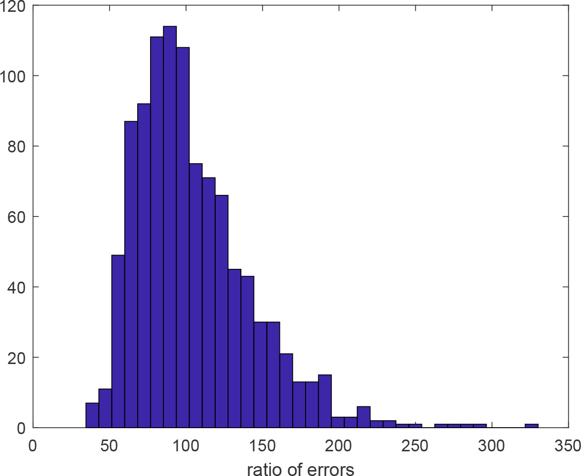
Figure 1.
A histogram of the ratio of the error of the most accurate prior product formula SS8s19 to our new solution, in the case without processing. The histogram is over the 1024 samples of 64 × 64 matrices. The average improvement is about a factor of 100, with the lowest being about 35.
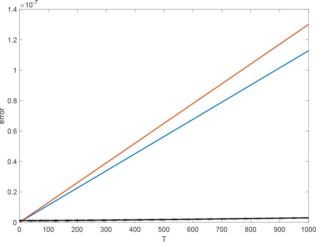
Figure 2.
The spectral-norm error for simulating an 8-qubit transverse-field Ising Hamiltonian in Eq. (59) for our product formula Y8m10b (black), SS8s19 (blue), and SS8s21 (red) from Ref. [29]. The size of the time step is 1, and the components of the Hamiltonian are normalised to unit norm.
Table 8.
The 8th order kernel tailored for large time step size t = 1.82 to improve the threshold.
| kernel for large time step | |
|---|---|
| w1 | 0.1777372900430394 |
| w2 | 0.2862580532195395 |
| w3 | 0.1701306063199336 |
| w4 | −0.3746748008394162 |
| w5 | 0.1485267804844835 |
| w6 | −0.3773225725485588 |
| w7 | 0.5395886879620081 |
| w8 | 0.2210419534887659 |
Table 9.
Comparison of constant factors ω for a selection of the lowest-error best product formulae for 6th order. We generate 1, 000 random Hamiltonians with d = 6 orbitals as in Eq. (60) and compute the average ω.
Table 10.
Comparison of constant factors ω for a selection of the lowest-error product formulae for 8th order. We generate 1, 000 random Hamiltonians with d = 6 orbitals as in Eq. (60) and compute the average ω.
Table 11.
Comparison of constant factors ω for a selection of the lowest-error product formulae for 10th order. We generate 1, 000 random Hamiltonians with d = 6 orbitals as in Eq. (60) and compute the average ω.
Table A1.
Comparison of constant factors ω for a selection of the lowest-error product formulae for 6th order. We generate 1, 000 random Hamiltonians with d = 4 orbitals as in Eq. (60) and compute the average ω.
Table A2.
Comparison of constant factors ω for a selection of the lowest-error product formulae for 8th order. We generate 1, 000 random Hamiltonians with d = 4 orbitals as in Eq. (60) and compute the average ω.
Table A3.
Comparison of constant factors ω for a selection of the lowest-error product formulae for 10th order. We generate 1, 000 random Hamiltonians with d = 4 orbitals as in Eq. (60) and compute the average ω.