
Table 1.
Comparison of previous results and our work on deterministic spatial search.
| Algorithms | Graph | Model | Number of marked vertices |
|---|---|---|---|
| Marsh and Wang [21] | 2 × n Rook graph | Alternating CTQW | Single |
| Qu et al. [22] | Star graph | Alternating CTQW | Single |
| Wang et al. [23] | Integer Laplacian spectra | Alternating CTQW | Multiple |
| Peng et al. [24] | Complete bipartite graph | Coined DTQW | Multiple |
| Our work | Complete bipartite graph | CTQW | Multiple |
Table 2.
Comparison of previous results and our work on spatial search on complete bipartite graphs.
| Algorithms | Model | Initial state | Success probability |
|---|---|---|---|
| Wong et al. [28] | CG framework for Laplacian walk | 1 (m, n → ∞) | |
| CG framework for adjacency walk | 1 (m, n → ∞) | ||
| Rhodes and Wong [29] | Coined DTQW | or (and 1 for a special case) | |
| (and 1 for a special case) | |||
| Xu et al. [30] | Coined DTQW | ≥ 1 − ɛ for any adjustable parameter ɛ | |
| Our work | CTQW | or | 1 |
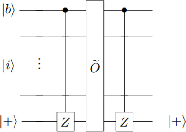
Figure 1.
Quantum circuit implementation for the oracle in (5)
| Algorithm 1 : Deterministic search algorithm on complete bipartite graphs. |
|---|
| Input: A complete bipartite graph Km,n with k marked vertices on the order-n part whose adjacency matrix is A, an oracle O that satisfies equation (5). |
| Output: A marked vertex. |
| 1: Calculate parameters and . |
| 2: Construct the initial state . |
| 3: Perform quantum walk search . |
| 4: Measure the final state and get |i〉. |
| 5: Return vertex i. |
| Algorithm 2 : Quantum Phase Estimation (QPE). |
|---|
| Input: A unitary U, initial state |0〉⊗p|ϕ0 (p is the number of qubits in the first register and |ϕ0〉 is an arbitrary state of the second register). |
| Output: An estimate θ̃ of one of the eigenphases of U. |
| 1: Apply Hadamard gate H to each qubit in the first register. |
| 2: Apply U2j on the second register controlled by qubit j, 1 ≤ j ≤ p in the first register. |
| 3: Apply inverse quantum Fourier transform to the first register. |
| 4: Measure the first register in the computational basis and get the result l. |
| 5: Return . |
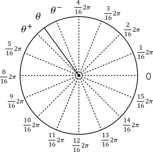
Figure 2.
The possible phase set returned by Algorithm 1 for M = 16. The best estimation for an angle θ is either θ+ or θ−.
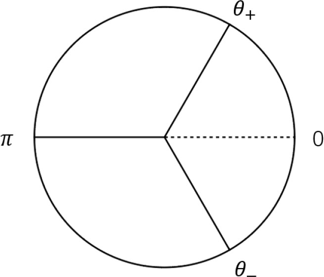
Figure 3.
The eigenphase distribution of U(t0) on the unit circle.
| Algorithm 3 : Quantum counting for search on complete bipartite graphs. |
|---|
| Input: Unitary U(t0), initial state|0〉⊗p|ψ〉 ( is the number of qubits in the first register and δ is the desired precision). |
| Output: Estimation k̃ of the number of marked vertices k with precision δ. |
| 1: Call Algorithm 2 and get the result θ̃. |
| 2: if θ̃ = π |
| then discard; |
| else |
| . |
| 3: Return k̃. |
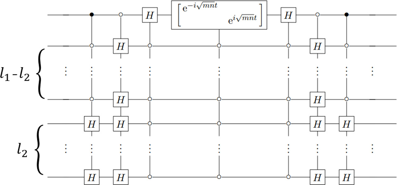
Figure 4.
Quantum circuit for implementation of e−iÃt.
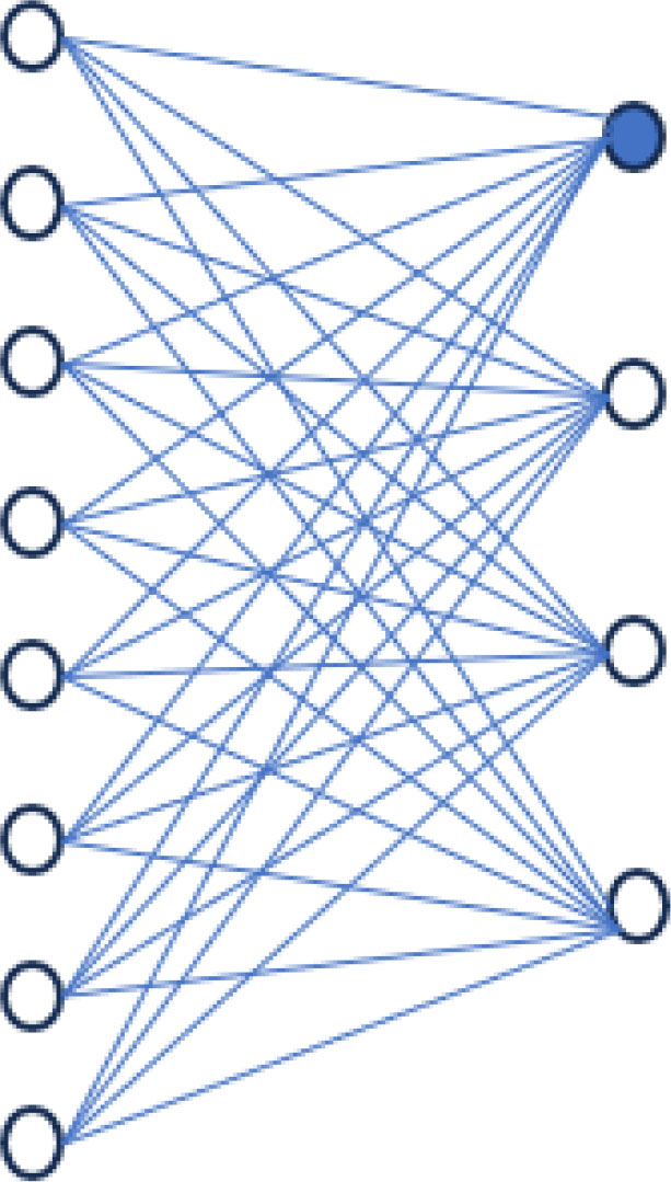
Figure 5.
Graph K8,4 with vertex |8〉 marked.
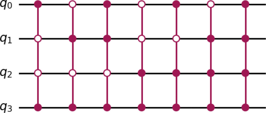
Figure 6.
Circuit simulation of the oracle for graph K8,4 with vertex |8〉 marked.
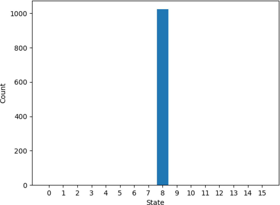
Figure 7.
State counts of the measurement result of the simulation.