
1. Introduction
Fault-tolerant control has emerged as a fundamental requirement in traction drive systems (Orlowska-Kowalska et al., 2022), representing vital components in electric vehicles and other high-dependability applications. These systems incorporate various subsystems, such as inverters, sensors, motors and control units, to ensure efficient, uninterrupted operation.
Modern fault-tolerant control (FTC) systems for electrical vehicles (EV) traction drives typically combine three coordinated stages: fault detection and diagnosis (FDD), fault isolation, and control reconfiguration. Over the past decade, significant research efforts have been devoted to the development of advanced FDD and FTC strategies for various fault scenarios in electric drives (Ahmed Baba et al., 2023; Bhuiyan et al., 2020; Gherghina et al., 2025; Khaneghah et al., 2023; Kumar et al., 2025; Li et al., 2025; Orlowska-Kowalska et al., 2022; Romdhane et al., 2026a,b). For instance, several studies have addressed inter-turn short-circuit (ITSC) faults in permanent magnet synchronous motors (PMSMs) using model-based, signal-based, and artificial intelligence techniques (Orlowska-Kowalska et al., 2022; Romdhane et al., 2026a,b; Zerdani et al., 2022; Zhang et al., 2025, 2023). Current, speed, and position sensor faults, including offset, gain, and complete signal loss, have also received considerable attention, with active FTC approaches based on observers, adaptive estimation, and neural networks (Adamczyk and Orłowska-Kowalska, 2023; Kommuri et al., 2016; Orlowska-Kowalska et al., 2022; Teler, 2026; Yousfi et al., 2009). Likewise, numerous contributions have focused on inverter switch faults, through fast detection algorithms and control reconfiguration methods (Altin et al., 2018; Bianchi et al., 2003a; De Araujo Ribeiro et al., 2004; Elsayed et al., 2022; Estima and Cardoso, 2012; Fadil et al., 2018; Hicham et al., 2017; Miraoui, 2025; Orlowska-Kowalska et al., 2022; Zerdani et al., 2019, 2021; Zhiduan and Lihao, 2024b). These studies demonstrate the growing interest in enhancing the reliability and availability of traction drive systems under a wide range of fault conditions.
The present study focuses on single-phase faults in drive systems, including loss of a phase-current measurement, failure of an inverter phase leg and loss of one motor phase. Once the faulty phase is identified and isolated, continued operation requires an alternative current path with an appropriate post-fault control strategy. Therefore, the converter topology plays a decisive role in determining the achievable performance under degraded operating conditions.
1.1. State of the art
Several fault-tolerant inverter configurations have been proposed to maintain the operation of electric drives after a single-phase fault (Mirafzal, 2014; Tousizadeh et al., 2019; Welchko et al., 2004; Zhang et al., 2021, 2014). Among the representative configurations reported in the literature are the switched-based four-leg inverter (SFI; Figure 1a), the capacitor-based four-leg inverter (CFI; Figure 1b), the switched-based four-leg neutral-point-connected inverter (SFNI; Figure 1c), and the capacitor-based four-leg neutral-point-connected inverter (CFNI; Figure 1d).
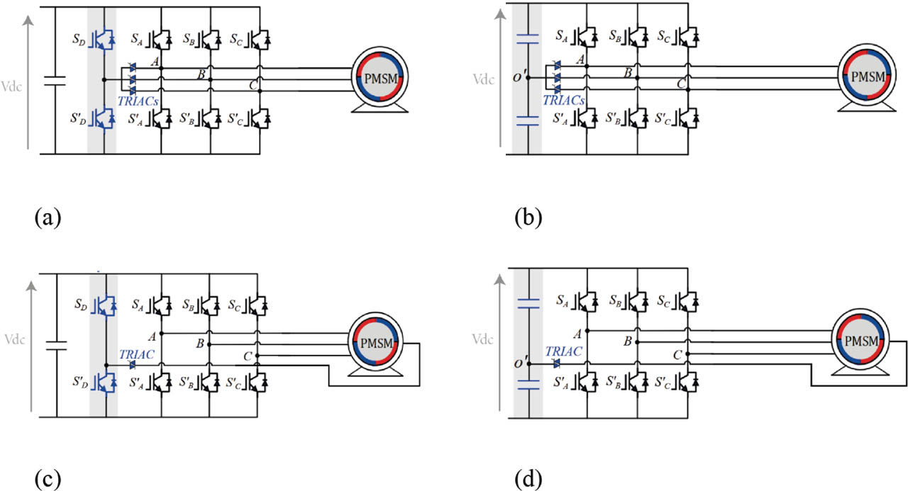
Figure 1.
Schematic of three-phase fault-tolerant topologies. (a) SFI. (b) CFI. (c) SFNI. (d) CFNI. CFI, capacitor-based four-leg inverter; CFNI, capacitor-based four-leg neutral-point-connected inverter; SFI, switched-based four-leg inverter; SFNI, switched-based four-leg neutral-point-connected inverter.
CFI topology has been extensively investigated for fault-tolerant operation (Fadil et al., 2018; Hang et al., 2023; Hicham et al., 2017; Huang et al., 2021; Hu et al., 2021; Li et al., 2019; Zerdani et al., 2019, 2021; Zhiduan and Lihao, 2024a; Zhu et al., 2017), whereas SFNI has been considered in previous fault-tolerant drive studies (Bianchi et al., 2003b; Bolognani et al., 1998; Kim and Sul, 2004; Meinguet and Gyselinck, 2009). In contrast, comparatively limited attention has been devoted to CFNI topology despite its reduced semiconductor requirements (Liu, 1993; Miraoui, 2025).
To clarify the trade-offs among these topologies, Table 1 summarizes the four representative configurations in terms of DC-bus structure, motor neutral accessibility, auxiliary semiconductor devices, semiconductor overrating cost factor (SOCF), post fault power ration factor (PPRF), attainable post-fault torque and fault-tolerant capability (Foster et al., 2010; Mirafzal, 2014; Tousizadeh et al., 2019; Welchko et al., 2004; Zhang et al., 2021, 2014).
Table 1.
Comparative analysis of SFI, CFI, SFNI, and CFNI topologies.
| TRIAC | IGBT | Inverter side | Motor side | ||||||
|---|---|---|---|---|---|---|---|---|---|
| SFI (a) | Non | Non | 3 | 2 | 1.83 | 1 | 1 | √ | × |
| CFI (b) | Oui | Non | 3 | 0 | 1.5 | 0.5 | 1 | √ | × |
| SFNI (c) | Non | Oui | 1 | 2 | 1.86 | 0.58 | 0.58 | √ | √ |
| CFNI (d) | Oui | Oui | 1 | 0 | 1.28 | 0.5 | 0.58 | √ | √ |
Here, PPRF denotes the maximum achievable post-fault apparent power normalised by the rated apparent power under healthy conditions. SOCF represents the weighted apparent power rating of the complete set of semiconductor devices normalised with respect to that of the six insulated-gate bipolar transistors (IGBT) in a conventional healthy three-phase inverter. The calculation assumes that each semiconductor device withstands a DC-bus voltage of 1 pu and conducts a phase-current root mean square (RMS) of 1 pu. Under these assumptions, the conventional healthy inverter exhibits an SOCF of 1.
The comparison highlights a fundamental compromise between post-fault capability and hardware complexity. The SFI preserves the rated torque but requires three triodes for alternating current (TRIAC) and two additional IGBTs, resulting in a relatively high SOCF of 1.83. The CFI eliminates the additional IGBTs and reduces the SOCF to 1.50, although its post-fault power capability is reduced. The SFNI can accommodate single-phase faults on either the inverter or motor side but requires additional semiconductor devices and exhibits the highest SOCF among the four topologies. In comparison, the CFNI requires only one auxiliary TRIAC and no additional IGBTs, yielding the lowest SOCF of 1.28 while retaining the capability to accommodate both inverter- and motor-side phase faults.
However, the CFNI presents some limitations. Its PPRF is reduced, especially under phase-loss (PL), and the post-fault torque and operation range are limited. In addition, the topology relies on a split DC bus and, therefore, requires sufficiently large DC-link capacitances to limit midpoint-voltage fluctuations. Despite these constraints, its low semiconductor count, structural simplicity, reduced SOCF and its capability to accommodate both inverter and motor-side phase faults make the CFNI particularly attractive for fault-tolerant traction applications where converter cost, volume and complexity are important considerations.
1.2. Research gap and motivation
Despite these attractive characteristics, fault-tolerant modulation and control of the CFNI topology have received considerably less attention than those of the CFI and SFNI configurations.
A recent work reported in Miraoui (2025) demonstrated the feasibility of fault-tolerant operation of a CFNI with PMSM under single-phase fault conditions using pulse width modulation (PWM)-based field-oriented control (FOC) methodology with adaptive reference adjustment. Building on these results, the present study further investigates the modulation stage by introducing a space vector pulse width modulation (SVPWM) strategy specifically adapted to the CFNI topology. SVPWM is selected because of its improved DC-link voltage utilisation and favourable harmonic performance, including reduced total harmonic distortion (THD), compared with conventional sinusoidal PWM (SPWM) (Kumar et al., 2010).
Under post-fault operation, each faulty phase leads to a specific voltage vector configuration and, consequently, to different sector definitions and switching sequences. Treating these three fault cases independently would require three distinct SVPWM algorithms.
These considerations motivate the development of a dedicated consolidated SVPWM framework for the CFNI topology, capable of handling the three phase-fault scenarios within a common formulation and thereby simplifying the modulation process. The proposed approach is conceptually inspired by the unified SVPWM strategy developed for the CFI topology in Zhiduan and Lihao (2024a).
1.3. Main contributions
To address the aforementioned research gap, this paper proposes a consolidated SVPWM-based framework for CFNI-fed PMSM drive under single-phase fault conditions. The main contributions are:
A systematic analysis of the CFNI post-fault voltage-vector configurations is carried out for faults affecting phases a, b, and c, allowing the corresponding sectors and admissible vectors to be identified.
A consolidated SVPWM formulation is developed for the CFNI topology, enabling the three phase-fault scenarios to be handled using a common modulation algorithm.
The consolidated SVPWM procedure is expressed through four computational steps analogous to conventional SVPWM, facilitating its integration into standard drive-control architectures.
A remedial FOC strategy combining the CFNI topology and the proposed consolidated SVPWM is developed to maintain PMSM operation following a single-phase fault.
The proposed method is evaluated through detailed simulation with particular attention to phase-current and torque responses, speed tracking and the THD of current and torque under healthy and post-fault operating conditions.
1.4. Paper organisation
The paper is organised as follows: Section 2 details the SVPWM methodology for CFNI topology under single-phase faults. The voltage-vector configurations, sector definitions, and switching sequences are first established for each phase-fault scenario. A consolidated SVPWM formulation is then developed to handle the three fault cases within a common modulation framework. The proposed procedure is finally summarised through four computational steps analogous to those of conventional SVPWM. Section 3 introduces a remedial strategy based on FOC, integrating the consolidated SVPWM and the CFNI topology to ensure reliable operation of the PMSM under faulty conditions. Section 4 provides a comprehensive simulation evaluation, demonstrating the proposed method's effectiveness in maintaining system functionality. Key findings are discussed in detail, along with potential limitations. Section 5 concludes the paper with a summary of contributions and implications of the proposed methodology.
2. SVPWM for Faulty Case
The development of the proposed SVPWM strategy for CFNI topology is inspired by the principles of conventional SVPWM for healthy operating conditions in a three-phase inverter, which have been extensively reported in the literature (Bin Ibrahim et al., 2014; Kumar et al., 2010; Shu et al., 2007; YingYing et al., 2011).
2.1. Sector of the reference voltage vector
Starting with the case of a fault in phase a, after detecting a failure, the damaged phase is electrically isolated; then, using the TRIAC, the neutral point is connected to the midpoint DC-link capacitor as shown in Figure 1d.
The model describing the three-phase output voltage is presented as follows:
Sa, Sb, and Sc represent the switching states of the three-leg transistors.
Considering the voltage oscillation at the capacitor midpoint and taking Δu as the voltage offset gives the expression of and .
The transformed a-b-c to α-β coordinates using Clarke transformation A with uan = 0 is expressed in Eq. (2).
Considering Eqs (1) and (2), the inverter's model in α-β coordinates is expressed in Eq. (3).
By combining the states of the four available inverter switches and, for simplicity in analysis and description, assuming Δu = 0, four voltage space vectors are obtained and their components are summarised in Table 2.
Table 2.
Available voltage vectors with neutral point connected to the midpoint of the DC-link capacitor and phase a eliminated.
| Sb | Sc | uα | uβ | Vx | Amplitude |
|---|---|---|---|---|---|
| 0 | 0 | Vdc/3 | 0 | V1 | Vdc/3 |
| 0 | 1 | 0 | V4 | ||
| 1 | 0 | 0 | V2 | ||
| 1 | 1 | −Vdc/3 | 0 | V3 | Vdc/3 |
For the cases of faults in b or c, and by following the same analysis used in a, we obtain four voltage space vectors as reported in Tables 3 and 4.
Table 3.
Available voltage vectors with neutral point connected to the midpoint of the DC-link capacitor and phase b eliminated.
| Sc | Sa | uα | uβ | Vx | Amplitude |
|---|---|---|---|---|---|
| 0 | 0 | −Vdc/6 | V1 | Vdc/3 | |
| 0 | 1 | Vdc/2 | V4 | ||
| 1 | 0 | −Vdc/2 | V2 | ||
| 1 | 1 | Vdc/6 | V3 | Vdc/3 |
Table 4.
Available voltage vectors with neutral point connected to the midpoint of the DC-link capacitor and phase c eliminated.
| Sa | Sb | uα | uβ | Vx | Amplitude |
|---|---|---|---|---|---|
| 0 | 0 | −Vdc/6 | V1 | Vdc/3 | |
| 0 | 1 | −Vdc/2 | V4 | ||
| 1 | 0 | Vdc/2 | V2 | ||
| 1 | 1 | Vdc/6 | V3 | Vdc/3 |
Based on the three summarised tables, the distribution of the basic voltage vectors in the α-β coordinate system is illustrated in Figure 2.
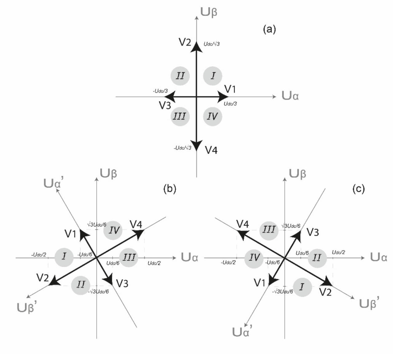
Figure 2.
Voltage vectors in the αβ plane. (a) Fault in a, (b) fault in b, and (c) fault in c.
2.2. Unification of the three cases
To address the complexity of implementing three separate SVPWM algorithms for each phase fault, a unified SVPWM approach is proposed in this section.
By comparing the three basic voltage vector distributions in Figure 2, it can be observed that they contain the same number of vectors with identical amplitudes, while differing only in the angular positions of the vectors in the αβ plane. Therefore, the three distributions can be expressed in a common α′β′ representation through an appropriate coordinate rotation. For the distribution in Figure 2a, no rotation is required and the α′β′ axes coincide with the original αβ axes. For Figure 2b, the α′β′ axes are rotated by with respect to the αβ axes, leading to the coordinate transformation given in Eq. (4). Similarly, for Figure 2c, the α′β′ axes are rotated by with respect to the original αβ axes, resulting in the transformation given in Eq. (5).
After these transformations, the three cases exhibit the same basic voltage vector distribution in the α′β′ plane, thereby enabling the development of a unified SVPWM approach.
In the sections that follow, we will present the additional steps required to complete the SVPWM process based on the common voltage vectors depicted in Figure 3.
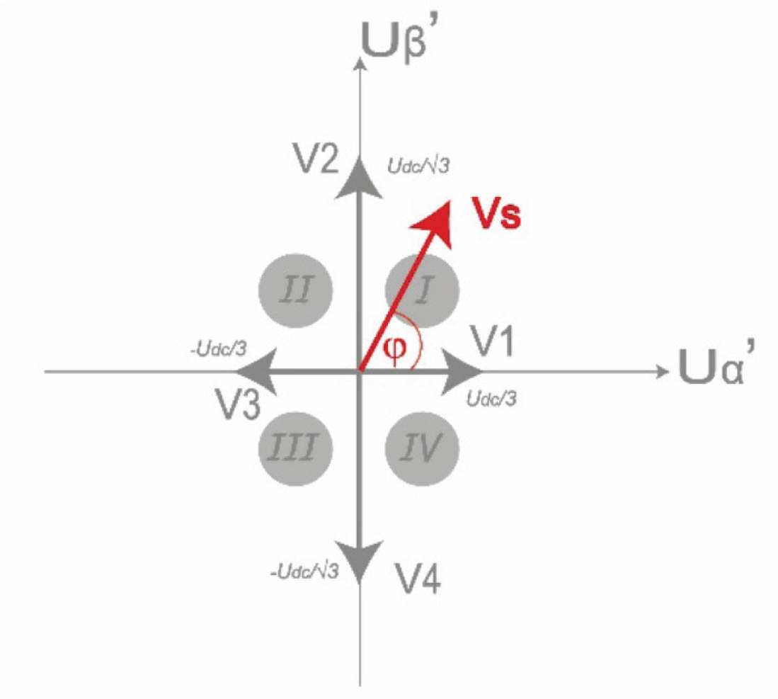
Figure 3.
Common voltage vectors in α′β′ plane.
2.3. Sector identification
The sector selection is determined according to the flowchart illustrated in Figure 4, based on the common voltage vectors in the α′β′ plane shown in Figure 3.
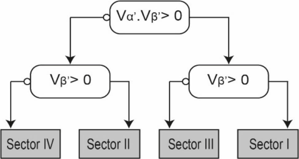
Figure 4.
Flowchart of sector identification.
2.4. Time calculation
The common space vector, as depicted in Figure 3, has only four distinct space vectors available. However, additional space vectors can be obtained by alternately applying active and zero vectors over the modulator's switching period Ts. For instance, the active vectors V1 and V2 can be combined to synthesise a reference space vector Vs with an angle between 0°and 90°.
Then the average space vector's amplitude can be expressed as:
with , and Ts = Tk + Tk+1 + T0.For any sector k (I, II, III, and VI), we can synthesise the reference space vector Vs using the following equation:
Now, based on Figure 3 and the analysis discussed earlier, we can derive the time calculations in Eq. (8)
with .It is essential to consider that the values of Vk and Vk + 1 vary across the sectors; therefore, the values of Tk and Tk + 1 for each sector are given in Table 5.
2.5. Switching sequence generation
To reduce switching losses, it is necessary to optimise the switching sequence. Figure 5 illustrates the possible switching sequences. As can be observed, the active vectors are selected by considering the switching states of the power switches in Table 2. Consequently, only one switch changes its state during each transition, thereby minimising switching losses.
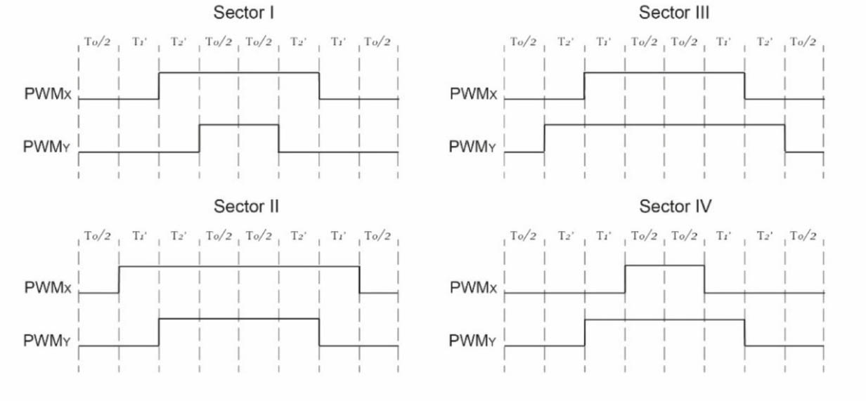
Figure 5.
Optimal switching patterns for the four sectors. PWM, pulse width modulation.
The notation (PWMx, PWMy) was adopted to provide a generalised formulation independent of the faulty phase. Specifically, under a phase-a fault, it corresponds to (PWMb, PWMc), under a phase-b fault, to (PWMc, PWMa), and under a phase-c fault, to (PWMa, PWMb). This notation was derived from the analysis of Tables 2–4, which led to the formulation of Table 6.
3. Control System Block Diagram
FOC is a widely used technique for managing a standard three-phase PMSM by separating the control of magnetic flux and torque via the d- and q-current axes (Chikh et al., 2011; Miraoui et al., 2025; Nicola et al., 2022). In this remedial strategy, as shown in Figure 7, the same FOC method is employed to produce the components Vd and Vq which are then transformed from the d-q to α-β coordinate system before being input into the consolidated SVPWM in Figure 6.
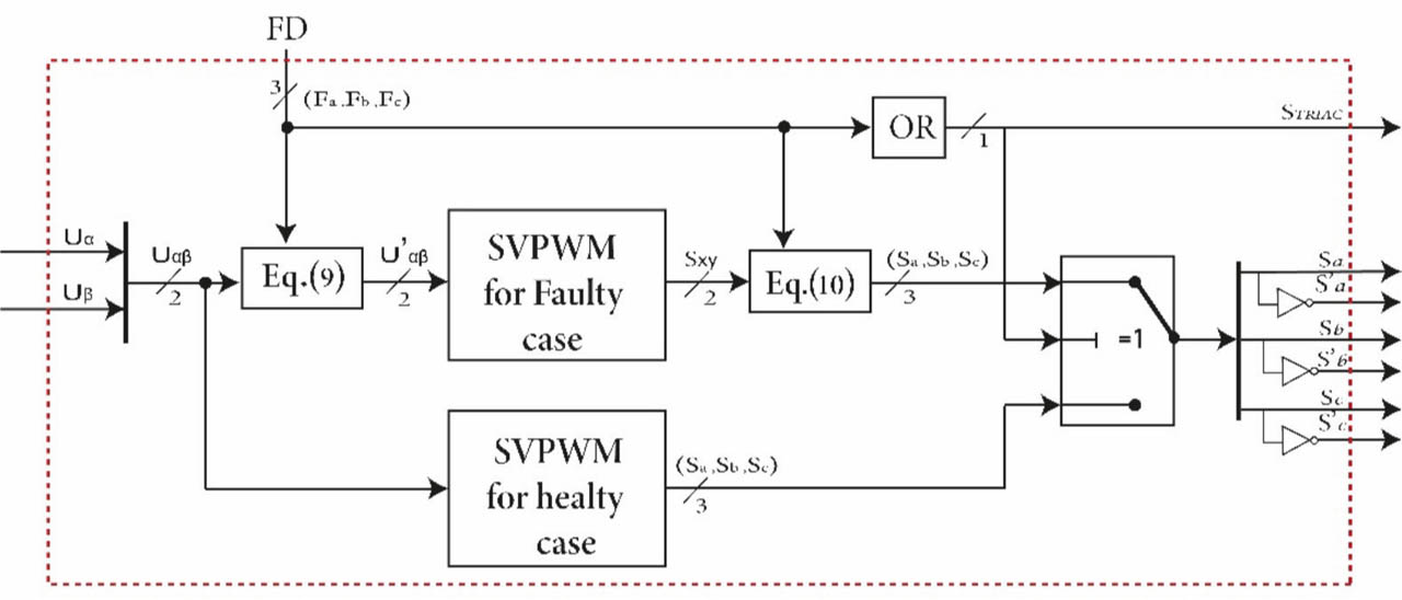
Figure 6.
Proposed consolidated SVPWM control block diagram. SVPWM, space vector pulse width modulation.
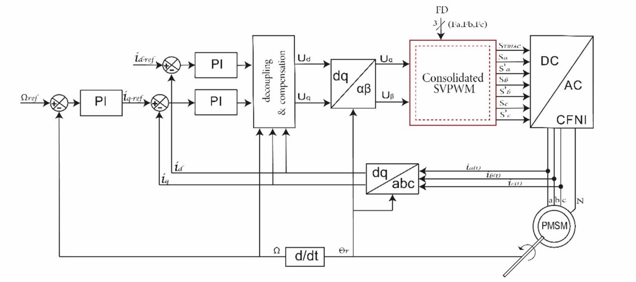
Figure 7.
Proposed single-phase FTC block diagram. CFNI, capacitor-based four-leg neutral-point-connected inverter; FTC, fault-tolerant control; PMSM, permanent magnet synchronous motor; SVPWM, space vector pulse width modulation; PI, proportional-integral.
As inputs Uα and Uβ are processed through the system, the conventional SVPWM directly generates the six switching signals under healthy operation. However, if a fault occurs and is detected, the fault detection signal, which is represented in Figure 6 by a three-bit signal fault detection (FD) (Fa, Fb, Fc ), activates the SVPWM algorithm for the faulty operation. Each bit identifies the corresponding faulty phase, where Fa, Fb, and Fc are associated with phases a, b, and c, respectively. Under a fault in phase a, only the bit Fa is set to 1.
In the faulty case, the processing is carried out using Uα′ and Uβ′ as inputs, obtained from Eq. (9). Eq. (9) combines the coordinate transformations introduced in Eqs (4) and (5) with the FD signal to automatically select the appropriate transformation according to the faulty phase. For example, when Fb = 1, Eq. (9) reduces to Eq. (4). Thus, regardless of the faulty phase, the voltage vectors are expressed in the common α′β′ reference frame shown in Figure 3.
The unified SVPWM generates the two switching signals Sx and Sy, which must be assigned to the two healthy phases according to the detected faulty phase. To map these output signals to the corresponding healthy phases, Eq. (10) is employed. This equation is derived from the relationships summarised in Table 6. For example, for a phase-b fault, Fb = 1, Eq. (10) gives Sc = Sx and Sa = Sy.
4. Simulation and Results
The proposed remedial strategy illustrated in Figure 7, together with the power configuration, was evaluated through a co-simulation approach using power simulation (PSIM) and MATLAB/Simulink (The MathWorks, MATLAB R2018b, United States). The control scheme was developed in MATLAB/Simulink, and the power structure was implemented in PSIM. The nominal ratings and parameters of the PMSM and CFNI used in the simulations are provided in Table 7.
Table 7.
System parameters.
| Parameters | Values |
|---|---|
| DC-voltage | 220V |
| Cbus | 4.4 mF |
| PWM frequency | 16 kHz |
| Rated power | 1,100 W |
| Rated speed | 3,000 rpm |
| Resistance and inductance | 2.875 Ω and 8.5 mH |
| Pole pairs | 4 |
| Viscous friction | 0.001 Nms |
| Rotational inertia J | 0.0008 kg·m2 |
| Permanent magnet flux | 0.175 Wb |
Three separate single-phase fault scenarios were considered by introducing a fault in phases a, b, and c. In each case, the fault was applied at t = 1 s. Following fault occurrence, the faulty leg was isolated, and the TRIAC shown in Figure 1d was triggered to connect the motor neutral point to the midpoint of the DC-link capacitors. Simultaneously, the consolidated SVPWM switches from the conventional SVPWM to the proposed post-fault modulation strategy.
The PMSM initially operated at a speed reference of 1,500 rpm and a torque reference of 1 Nm. At t = 2 s, the torque reference was increased from 1 Nm to 2 Nm. Additional speed reference variations were then applied under post-fault operation to evaluate the performance of the proposed strategy at different operating points. The following analysis separately evaluates the speed, torque, and current performances using quantitative indices in addition to the time-domain responses.
Figure 8 presents the rotor-speed response before and after fault occurrence. Under healthy operation, the measured speed follows the reference at 1499.8 rpm, corresponding to a relative error of 0.013%.
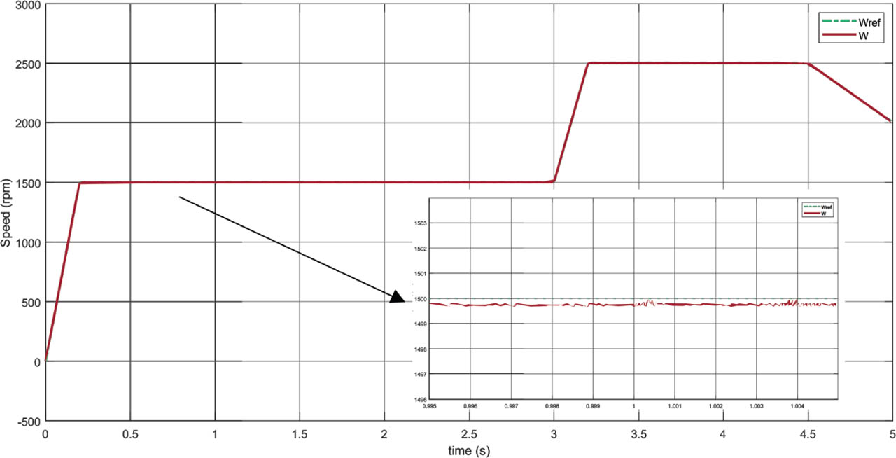
Figure 8.
Speed response before and after a fault occurs in phase a at 1 s.
The enlarged view at 1 s shows that the transition from healthy to post-fault operation introduces a very small perturbation, and the speed remains tightly regulated around its reference immediately after reconfiguration.
Furthermore, as shown in Figure 8, the PMSM continues to follow the changes of the speed reference from 1,500 rpm to 2,500 rpm and later to 2,000 rpm, demonstrating that the proposed approach preserves the speed tracking capability after fault accommodation.
Figure 9 presents the rotor torque response under healthy and faulty conditions. The torque follows the 1 Nm reference with a mean value of 1.003 Nm under healthy operation and 0.9999 Nm after fault reconfiguration, confirming the capability of the proposed strategy to preserve the average torque production.
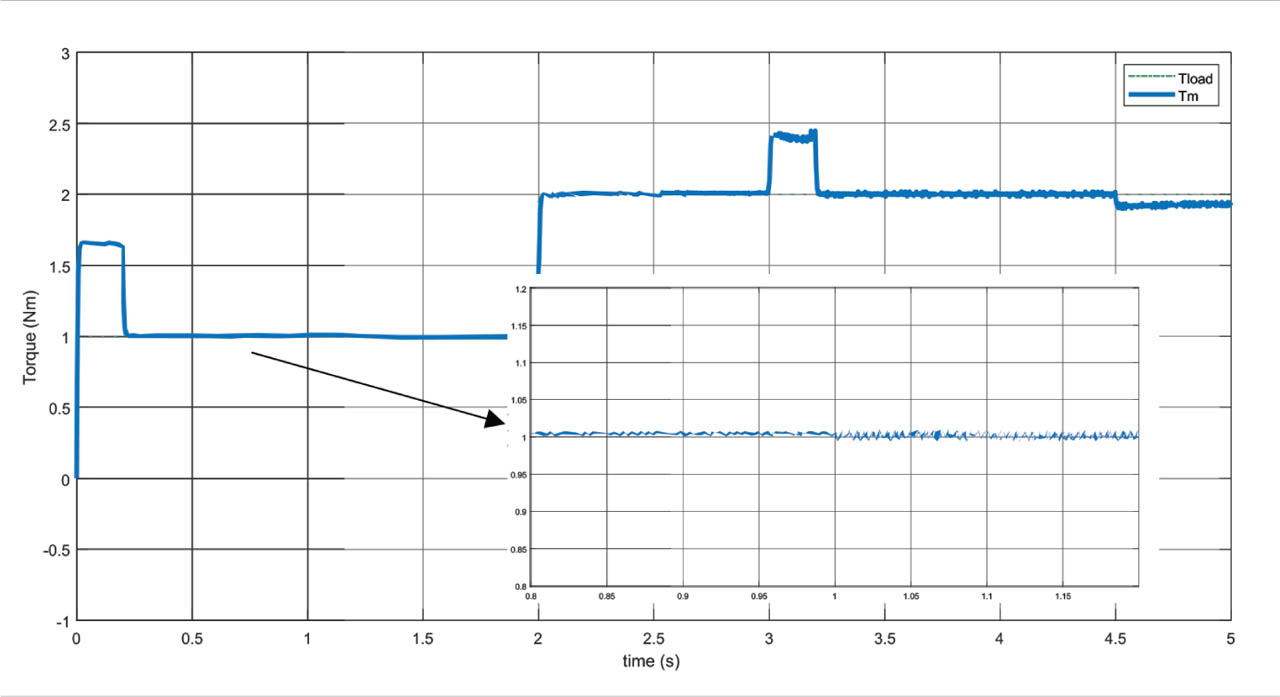
Figure 9.
Torque response before and after a fault occurs in phase a at 1 s.
The main post-fault effect is, therefore, an increase in torque oscillations: the torque ripple increases from approximately 0.56% to 1.61%, while the torque distortion rises from 0.14% to 0.33%. Nevertheless, the torque reference remains accurately tracked after the load increase to 2 Nm at t = 2 s.
Figure 10 presents the phase and neutral currents for faults occurring in phases a, b, and c. Before the fault, the three-phase currents are balanced. After reconfiguration, the current of the faulty phase is suppressed while the two healthy phase currents are increased and the neutral current becomes the sum of the two healthy phase currents.
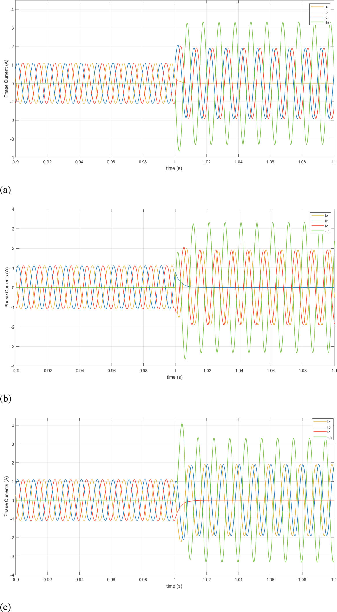
Figure 10.
Current response before and after a fault occurs at 1 s, (a) in phase a, (b) in phase b, and (c) in phase c.
Table 8 summarises the current amplitudes and phase displacements before and after fault occurrence in the three fault scenarios.
Table 8.
Current amplitudes and phase displacements in the three faulty scenarios.
| Amp. | Deph. | Amp. | Deph. | Amp. | Deph. | Amp. | Deph. | |
|---|---|---|---|---|---|---|---|---|
| ia | iN | 0 | 0 | - | ||||
| ib | iN | 0 | - | |||||
| ic | iN | 0 | - | |||||
| in | 0 | - | 3iN | 0 | 3iN | 0 | 3iN | 0 |
In line with observations in the literature (Bianchi et al., 2003b; Bolognani et al., 1998; Kim and Sul, 2004; Liu, 1993; Meinguet and Gyselinck, 2009), the phase-current displacement is reduced to one-sixth of a period, while the amplitude of the current increases from 1.105 A to 1.909 A, corresponding to approximately 1.73 times the healthy value. Additionally, the amplitude of the neutral current reaches 3.315 A, three times higher than the phase currents under normal operation. This increase results from the need to maintain electromagnetic torque after the loss of one phase, requiring the two remaining healthy phases to carry higher currents.
The harmonic quality of the currents was evaluated through FFT analysis, as shown in Figure 11. The results show that the current THD remains below 1%, with a value of 0.28% for a speed of 1,500 rpm.
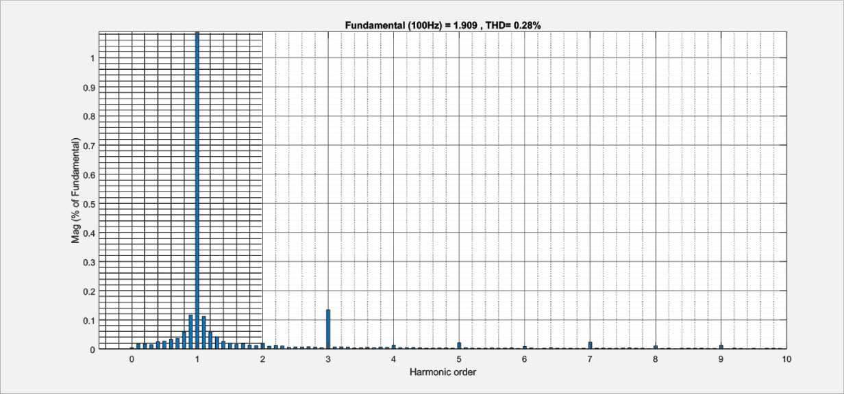
Figure 11.
Current THD in faulty case. THD, total harmonic distortion.
The combined speed, torque and current results confirm the effectiveness of the proposed remedial strategy. In terms of practical limitations, maintaining the increased post-fault current levels for extended durations may require oversizing of the inverter switches and leads to increased copper losses in the motor. Alternatively, the allowable peak currents of both the inverter and the motor, together with their permissible overload durations, must be considered. As these limits are approached, a smooth transition towards a degraded operating mode should be applied to avoid an abrupt torque loss, while protecting the drive from excessive electrical and thermal stress.
From an implementation perspective, this unified approach reduces the number of required SVPWM algorithms from four to two. Without consolidation, the complete controller would require one conventional SVPWM for healthy operation and three dedicated SVPWM algorithms corresponding to the three possible faulty phases. This consolidation reduces the number of algorithms and simplifies the control architecture. Since the present study is simulation-based, no specific digital processor is considered; therefore, execution time and memory savings are not quantitatively reported.
5. Conclusion
This paper presented a single-phase FTC strategy applicable to traction drive systems, employing a consolidated SVPWM technique dedicated to a CFNI. The proposed approach unifies the modulation process for faults occurring in phases a, b, and c, thereby avoiding the use of three separate fault-dependent SVPWM algorithms and simplifying the control implementation.
This method was demonstrated through simulations on a PMSM considering faults independently occurring in phases a, b, and c. Simulation results confirmed that, after fault detection and converter reconfiguration to eliminate the faulty phase, the torque production and speed tracking are maintained continuously. The two healthy phase currents increase to approximately 1.73 times their healthy state value, with the required phase displacement, while the neutral current ensures the return path. The proposed approach also preserves good waveform quality under post-fault operation; current THD remains below 1% in the investigated operating conditions. The results obtained under load and speed variation further demonstrate the ability to maintain stable operation.
Nonetheless, maintaining the increased post-fault currents for extended periods may require oversized inverter switches and lead to higher motor copper losses. Otherwise, overload capability and permissible duration must be considered. Once these limits are attained, a smooth transition towards a degraded operation mode should be applied to avoid abrupt torque loss and excessive electrical and thermal stress.
Overall, the proposed consolidated SVPWM provides an effective solution for fault-tolerant operation of CFNI-based PMSM traction drive systems. Future work could focus on experimental validation across different motor types and, therefore, extend the approach to other high-dependability applications.