
1. Introduction
DC gear motors are used in applications that require high torque and precise low-speed control (Reyes-Reyes et al., 2010; Verstraten et al., 2015). They are important in robotics and automation for driving mobile platforms and joints with stable motion. In industry, the power conveyor systems, packaging machines and actuators for cost-effective continuous operation. They are also used in medical devices, such as infusion pumps and adjustable beds, where precision is critical. They are also used in consumer electronics and renewable energy systems, such as solar trackers, which require accurate positioning and energy efficiency. A DC gear motor is an integrated electromechanical device that combines a brushed DC motor and a gear reduction mechanism (Hsueh and Fazdi, 2026; Kim et al., 2025). The gearbox reduces the motor’s high rotational speed and increases its output torque, making it suitable for driving loads such as robot wheels, conveyor systems and positioning mechanisms.
Iterative learning control (ILC) is a technique of performing a task repeatedly and updating the control input at every iteration according to a given learning law. In each iteration, the control action for the next trial is adjusted based on the tracking error of the previous trial. With the increase in the number of iterations, the tracking error is gradually decreased. It can perform high-precision trajectory tracking in the presence of non-linearities, uncertainties and modeling inaccuracies. Due to its efficiency in repetitive tasks, ILC has been widely applied in robots, industrial automation, CNC machines, precision motion systems, autonomous vehicles and batch processes. Therefore, ILC has been an important intelligent control strategy for repetitive electromechanical and industrial applications (Ahn et al., 2007; Bukkems et al., 2005; Ha et al., 2025).
ILC can be classified from several complementary perspectives. This reflects the evolution of ILC from a simple error-driven learning strategy to a versatile framework that can be applied to complex and uncertain systems. In terms of system knowledge, ILC methods are generally classified into model-based, model-free (data-driven) and hybrid approaches. The model-based ILC exploits the mathematical model of the system to design the learning law and guarantee the convergence. However, accurate models are usually hard to obtain in non-linear or industrial environments; thus, data-driven approaches, such as the model-free adaptive ILC (MFAILC) and data-driven ILC (DDILC), have been developed (Cao et al., 2025; Chi et al., 2025; Meindl et al., 2025). In these approaches, control laws are constructed directly from input-output data without requiring explicit system models. Hybrid frameworks such as iterative model learning (IML) and dual ILC (DILC) combine the benefits of both paradigms by enabling simultaneous model learning and control learning, thus improving flexibility and performance (Chen et al., 2023; Feng et al., 2023; Xu et al., 2026).
According to the application of the knowledge of previous iterations, ILC can be classified into several types from the point of view of the learning mechanism. The conventional ILC updates the control input based on past tracking errors and gradually reduces the error over repeated trials (Ahn et al., 2007; Bukkems et al., 2005). Adaptive iterative learning control (AILC) (Chen et al., 2023; Feng et al., 2023; Ha et al., 2025; Xu et al., 2026) is developed to handle uncertainties and disturbances, where the parameter adaptation laws are used to improve the robustness in non-linear and time-varying systems. Also, intelligent learning techniques have been integrated, such as the neural network-based ILC, where the unknown non-linear dynamics are approximated and iteratively improved (Li et al., 2025). More advanced schemes are predictive ILC that consider constraints and varying operating conditions (Yu et al., 2026) and sliding mode ILC that increases robustness to non-linearities and disturbances via discontinuous control action (Zhou et al., 2024).
Based on the control structure, the ILC systems can be divided into feedback and parameter learning. In feedforward ILC, the learned signal is directly used as the control input for the future iterations. In practical applications, a combination of feedback control (such as proportional-derivative [PD] or PID controllers) and iterative learning is often used to ensure stability and improve transient performance, especially when there are disturbances or communication constraints (Shen et al., 2025; Xu et al., 2026). Parameter-learning ILC updates the controller parameters rather than the control signal accumulation, which is beneficial for systems with input saturation or physical constraints (Zhou et al., 2024).
ILC can also be categorised based on system dynamics and uncertainty properties. The early work in ILC was mainly on linear systems because they are mathematically easier to analyse and have better convergence properties. But nowadays ILC methods are increasingly applied to non-linear, time-delay and uncertain systems, for which robustness, adaptivity and stability are crucial for reliable operation (Cao et al., 2025; Chen et al., 2023). In addition, constrained ILC approaches have been developed to handle practical implementation issues such as actuator saturation, limited control inputs, varying iteration lengths and changing reference trajectories. These developments significantly enhance the applicability of ILC in real industrial and electromechanical systems (Shen et al., 2025).
ILC is traditionally formulated in the time domain, where it is assumed that each task is repeated over a fixed time interval in the domain of operation. But this assumption has recently been relaxed. Spatial ILC (SILC) redefines the learning process in the spatial domain, which enables the variations of the execution speed with a guaranteed learning convergence (Yang et al., 2022). Additionally, intermittent ILC has been suggested for networked control systems with packet dropouts and communication constraints, where learning is preserved despite missing data (Xu et al., 2026). These extensions greatly increase the applicability of ILC in the fields of robotics, manufacturing and networked environments.
Despite the remarkable progress in ILC, the selection of suitable learning gains is still a difficult problem. Conventional gain tuning is generally performed using trial-and-error or conservative analytical methods, which can result in suboptimal performance for non-linear and uncertain systems. In addition, many optimisation algorithms involve large numbers of iterations and great computational effort, which limits their suitability for real-time embedded applications. Most of the existing studies are focussed on the optimisation of the parameters of the PID controller, while the intelligent tuning of the learning gains of the ILC has received relatively little attention (Son et al., 2025). In this study, a DC gear motor is controlled by a PD-type of ILC scheme. Optimal controller gains are learned from non-linear mapping between system performance indices and optimal controller gains using a Bayesian neural network (BNN), which calculates proportional and derivative learning gains (Bishop, 1995; Nabney, 2002). The BNN is trained for optimal gain tuning of the BNN-ILC controller on a dataset generated under different operating conditions. The proposed method reduces the manual tuning efforts and improves tracking accuracy, convergence speed and robustness against disturbances and modelling uncertainties.
The remainder of this paper is organised as follows. The DC gear motor system is represented by the transfer function in Section 2. Section 3 describes the basic concept and operation principle of the ILC scheme, including the learning mechanism for improving the tracking performance in the next iteration. In Section 4, the theory of BNNs for regression is described in detail. Section 5 presents the experimental setup and implementation procedure, including DC gear motor control system, data generation process, BNN training and ILC controller deployment. Also, this section includes experimental and simulation results, performance evaluation and discussions. Finally, Section 6 concludes this paper by summarising the main contributions and findings of this work and giving recommendations for future research directions in intelligent control and learning-based motor control systems.
2. Transfer Function of DC Gear Motors
The mathematical model of DC gear motors is derived from the electrical dynamics of the brushed DC motor, the mechanical dynamics of the rotor and load, and the kinematic relation introduced by the gearbox.
The electrical equation is given by:
The mechanical equation has the following form:
where:Va (t) : the armature voltage (V),
ia (t) : the armature current (A),
ωm (t) : the angular velocity of the motor (rad/s),
Ra : the armature resistance (Ω),
La : the armature inductance (H),
Ke : the back electromotive force (back-EMF) constant (V · s/rad),
Kt : the torque constant (N · m/A),
Jeq : the reflected inertia at the motor shaft (kg · m2),
Bm : the viscous friction (N · m · s).
The electrical equation in the Laplace domain is as follows:
where s is the Laplace operator.The mechanical equation in the Laplace domain is given by:
By setting TL = 0, the transfer function of the DC motor is given by:
The relationship between the armature voltage and the output angular velocity of the gear box is given by:
where ω0 (s) is the output angular velocity of the gear box and N is the ratio of the gear box.The electrical and mechanical dynamics of the DC motor are also characterised by two different time constants as follows:
where:τe : the electrical time constant (s),
τm : the mechanical time constant (s).
The electrical time constant τe represents the time required for the armature current to reach approximately 63.2% of its steady-state value following a step voltage input. Similarly, the mechanical time constant τm represents the time required for the motor speed to reach approximately 63.2% of its steady-state value.
For most small DC motors, the electrical time constant is much smaller than the mechanical time constant; therefore, the difference between these time constants can be expressed as follows:
After a very short transient, the current can be approximated by its quasi-steady-state value obtained from the electrical Eq. (1). Since τe ≪ τm, the current derivative is negligible compared with the resistive term:
Therefore, Eq. (1) yields:
Eq. (11) in Laplace domain is given by:
Substituting Eq. (12) into Eq. (4) and letting TL = 0 results in:
Therefore, the transfer function of the DC gear motor is given by:
In this study, a DC chopper is used to regulate the motor current. Therefore, the transfer function from the duty cycle of the chopper to the output speed of the gear motor is given by:
where D (s) is the duty cycle of the chopper and Eq. (15) represents a first-order system.3. ILC
ILC is a control methodology that has been developed for systems that repeat the same task over a finite time interval. The basic idea of ILC is that the information from past executions, called iterations or trials, is used to improve the tracking performance in the following operations.
The output of an ILC controller is given by:
where:ek (t) = rk (t) − yk (t) : the tracking error at the k - th iteration,
uk (t) : the control input at the k - th iteration,
uk+1 (t) : the control input at the k + 1 - th iteration,
L : the learning function.
The PD-type ILC update law is given as follows:
where:KP,ILC: the proportional learning gain,
KD,ILC: the derivative learning gain.
The Laplace transform of Eq. (17) is given by:
where s = jω is the Laplace operator.The z-transform of Eq. (18) is given by:
where z = ejωTs is the z operator and Ts is the sampling interval.Eq. (19) can be written as follows:
The system converges if the following condition is satisfied:
At a DC condition, ω = 0 and L(z) = KP, ILC, the following condition must be satisfied:
where G(0) is the DC gain of the transfer function of the controlled plant.From Eq. (23), the value of KP, ILC should be chosen so that:
Alternatively, the value of KP, ILC is chosen as follows:
At a high-frequency condition, ω = π/Ts, therefore z = ejωTs = ejπ = −1 and L (z) in Eq. (21) yields:
The system is stable if the following condition is satisfied:
Using Eqs (26) and (27) gives:
Eq. (28) can be also written as follows:
4. BNNs for Regression
4.1. Principle of bayesian inference
BNNs are an extension of standard neural networks where the weights and biases are no longer deterministic fixed values but probability distributions. The probabilistic framework enables the network to quantify uncertainty of its predictions, which is very important in applications of engineering, control and decision-making where reliability and robustness are needed. For regression problems, BNNs give predictive distributions with mean and variance, and for classification tasks, they estimate class probabilities for each class. BNNs improve generalisation and reduce overfitting by using Bayesian inference.
Applying Bayes’ theorem yields the posterior distribution of a neural network’s weights and biases given a dataset, as follows:
where w is the vector of weights and biases and p (w | D) is the posterior distribution of weights and biases. p (w) is the prior distribution of weights and biases and p (D | w) is the dataset likelihood. Finally, p (D) is a normalisation factor ensuring the posterior distribution integrates to 1. p (D) is also known as evidence.4.2. Bayesian model comparison
The use of Bayesian inference enables the handling of network complexity. More complex networks typically contain a greater number of hidden nodes. To clarify this, suppose that several neural networks (Xi) are compared and ranked using Bayesian model comparison as follows:
In Eq. (31), the prior distribution p (Xi) is the same for all the networks. The normalisation factor p (D) does not depend on the network. Therefore, the evidence p (D | Xi) can be used to select the best network architecture. In particular, the optimal number of hidden nodes can be determined based on the maximum value of the evidence p (D | Xi).
4.3. Bayesian network regularisation
In neural network training, regularisation is required to prevent the weights and biases from becoming excessively large, which can lead to overfitting and poor generalisation. Therefore, instead of using only a data error function, a weight penalty term is added to form a cost function, expressed as follows:
where:ED (w) : the data error function,
EW (w) : the weight function,
z (xn; w) : the network output corresponding to the n - th pattern of the training data,
tn : the target corresponding to the n-th pattern of the training data,
W : the number of network weights and biases,
α and β : The hyperparameters.
The cost function Eq. (32) is derived based on the assumption of a Gaussian approximation for the prior and posterior distributions of the network weights and biases. The hyperparameters α and β can be found by utilising the evidence procedure, which is an iterative algorithm for determining the optimal values of the weights and hyperparameters given a training dataset. By applying Bayes’ theorem again, the posterior distribution of the hyperparameters given a dataset D can be expressed as follows:
4.4. The evidence procedure
In the evidence procedure, there is a need of maximising p (D | α, β). This term can be found by integrating data likelihood over all possible weights as follows:
According to Bishop, (1995); Nabney, (2002), instead of directly computing the evidence Eq. (24), it is more convenient to evaluate the log evidence as follows:
where:wMP : the most probable vector of network weights and biases,
W : the number of network weights and biases,
N : the number of patterns in the dataset,
A : the Hessian matrix (second-order derivative matrix) of the cost function.
The Hessian matrix A is computed as follows:
where:∇∇H (wMP) : the Hessian matrix of the data error function ED (w) at wMP,
I : the identity matrix,
W : the number of weights and biases.
The log evidence can be used to rank different network architectures, such as those with varying numbers of hidden nodes. The optimal number of hidden nodes corresponds to the highest value of the log evidence.
By taking partial derivative of Eq. (37) with respect to α and β, and letting them to be equal to zero, the values of α and β can be determined according to re-estimation periods of α and β as follows:
where γi (i = 1,…W) are the eigenvalues of the data function ED. The term γ is used to measure the number of well-determined parameters in the network (Bishop, 1995; Nabney, 2002).5. Experiment
5.1. Hardware and software
Figure 1 shows the overall experimental system of the DC gear motor control. Figure 2 shows the block diagram of the experimental setup. The experimental system consists of a laptop with data acquisition (DAQ) software, an Arduino Nano board, a DC chopper, 12 VDC power module and a DC gear motor with an encoder. In this study, a JGA25-370 12 V encoder gear motor is used as an experimental plant. This motor is a widely used brushed DC geared motor equipped with an integrated incremental Hall-effect encoder that provides speed and position feedback. Its typical specifications are summarised in Table 1.
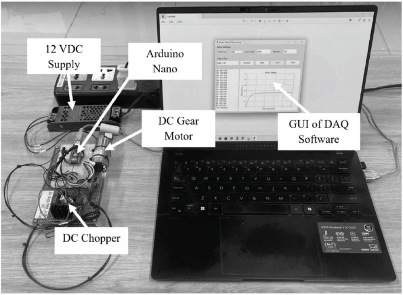
Figure 1.
The experimental system. DAQ, data acquisition; GUI, graphical user interface.
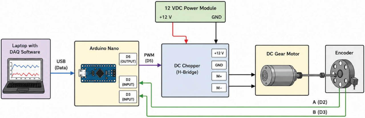
Figure 2.
Block diagram of the experimental system. DAQ, data acquisition.
Table 1.
Typical specifications of the JGA25-370 12 V encoder gear motor.
| Motor type | Brushed DC gear motor |
|---|---|
| Rated voltage | 12 V DC |
| Motor diameter | 25 mm |
| Motor model | 370 |
| Encoder type | Quadrature Hall-effect encoder |
| Encoder channels | A and B (90° phase shift) |
| Encoder supply voltage | 3.3–5 V DC |
| Encoder pulses | Usually 11 pulses/revolution (PPR) at the motor shaft |
A USB interface is used for data transfer and monitoring between the laptop and the Arduino Nano. The control signal for the armature voltage supplied to the DC gear motor is provided to the DC chopper through pin D5 by the pulse-width modulation (PWM) control signal produced by the Arduino Nano. The 12 VDC power module supplies power to the DC chopper and motor drive system. Mounted on the shaft of the DC gear motor is the encoder which provides feedback signals for the motor speed and rotational position. The encoder outputs are connected to the D2 and D3 pins of the Nano Arduino to measure the speed of the acquisition and to acquire the feedback.
The graphical user interface (GUI) of the DAQ software developed for the experimental system is shown in Figure 3. The GUI can display and plot the motor speed response in real time, allowing the user to continuously monitor the operating condition and dynamic performance of the DC gear motor during the experiment. The real time visualisation feature allows to observe important characteristics of the motor response such as transient behaviour, steady state speed, rise time, overshoot and speed fluctuations with different operating conditions and control inputs. Apart from the real time monitoring, the DAQ software is equipped with the data acquisition and recording ability to record the motor speed response data over the course of the experiment. The acquired data can be exported and processed in MATLAB for further investigation and offline analysis. This offline analysis can be used for various purposes such as system identification, mathematical modelling, parameter estimation, controller tuning and performance evaluation of the control system of the DC gear motor. Also, the recorded experimental data can be used to verify theoretical models and to develop advanced control strategies to enhance the dynamic performance and robustness of the motor drive system.
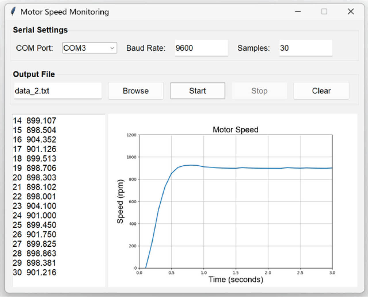
Figure 3.
GUI of the DAQ software. DAQ, data acquisition; GUI, graphical user interface.
5.2. Data generation
Figure 4 shows the speed response in revolutions per minute of the DC gear motor to a 0%–100% duty cycle step change. This experiment was carried out to determine the dynamic behaviour of the motor and to obtain a mathematical model suitable for controller design and performance evaluation. The response of the measured response indicates that the motor speed increases gradually from the initial steady state value to the final steady state value, a typical feature of a first order dynamic system.
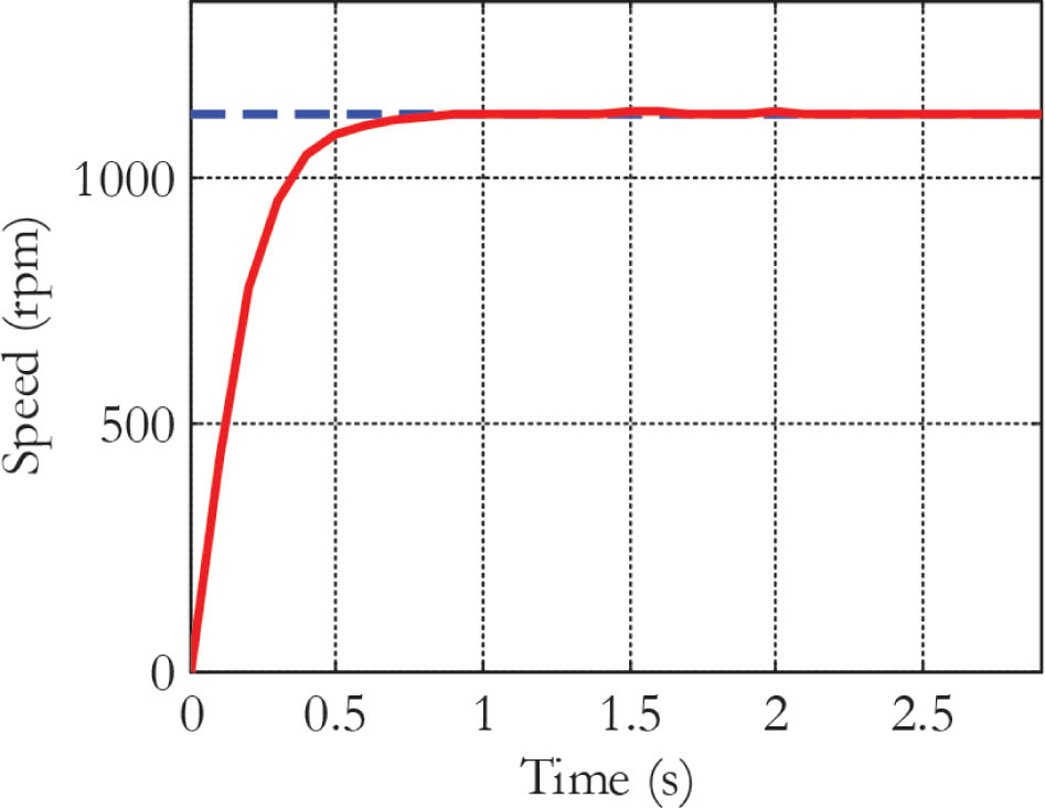
Figure 4.
Speed response of the DC gear motor to a step input in duty cycle from 0% to 100%.
A transfer function of the DC gear motor was identified using the experimental input–output data with the System Identification Toolbox in MATLAB. The speed response data were fitted to the first order model structure to estimate the system gain and time constant. The obtained transfer function is a simple approximation and can be used for simulation, system analysis and controller design. In particular, the approximate transfer function of the motor is given by:
In this study, the conventional proportional-integral (PI) controller is used only as a baseline controller for comparison purposes. This controller is employed only to evaluate the performance improvement achieved by the proposed method. The gains of the PI controller are determined from the transfer function given in Eq. (41) using the ‘pidtune’ function in MATLAB. The ‘pidtune’ function is a model-based frequency-domain control design algorithm that automatically computes the controller parameters based on the dynamic model of the plant. Specifically, it analyses the open-loop frequency response of the transfer function and employs loop-shaping techniques to determine the controller gains that achieve an appropriate balance between transient performance and robustness. The algorithm selects a suitable gain crossover frequency and phase margin, typically around 60°, to ensure closed-loop stability while providing a fast dynamic response, satisfactory disturbance rejection and minimal overshoot. For digital control applications, ‘pidtune’ also accounts for the specified sampling interval and directly computes the corresponding discrete-time controller parameters. In this study, a PI controller is adopted; therefore, only the proportional gain and the integral gain are optimised, while the derivative gain is omitted. After applying the ‘pidtune’ algorithm to the transfer function in Eq. (42), the controller gains are obtained as follows: KP, PI = 0.041 and KP, PI = 0.813.
The z-transform of Eq. (42) with a sampling interval of 0.1 s is given by:
Eq. (43) is equivalent to:
The discrete-time form of Eq. (44) is given by:
where:nk : the motor speed at the k -th sampling instant,
nk −1 : the motor speed at the k − 1 -th sampling instant,
Dk −1 : the duty cycle at the k − 1 -th sampling instant.
If the duty cycle remains unchanged, then Eq. (45) becomes:
The output of the discrete-time PD-type ILC controller is given by:
where:ek : the tracking error at the k -th sampling instant,
ek −1 : the tracking error at the k − 1 -th sampling instant,
KP, ILC : the proportional gain,
KD, ILC : the derivative gain,
Ts : the sampling interval.
The dataset is built with Eqs (46) and (47) for different motor operating conditions with the ILC controller. Figure 5 shows the flowchart for dataset generation using MATLAB. The parameters and storage vectors are initialised first, and the parameter vectors a and b are generated. Then the algorithm iterates through all possible combinations of a and b in nested loops. For each combination the ‘ILC_model’ function is executed, and the settling time and overshoot are saved together with the corresponding controller parameters. The generated dataset is saved in ‘ILC_data.mat’ after evaluating all combinations.
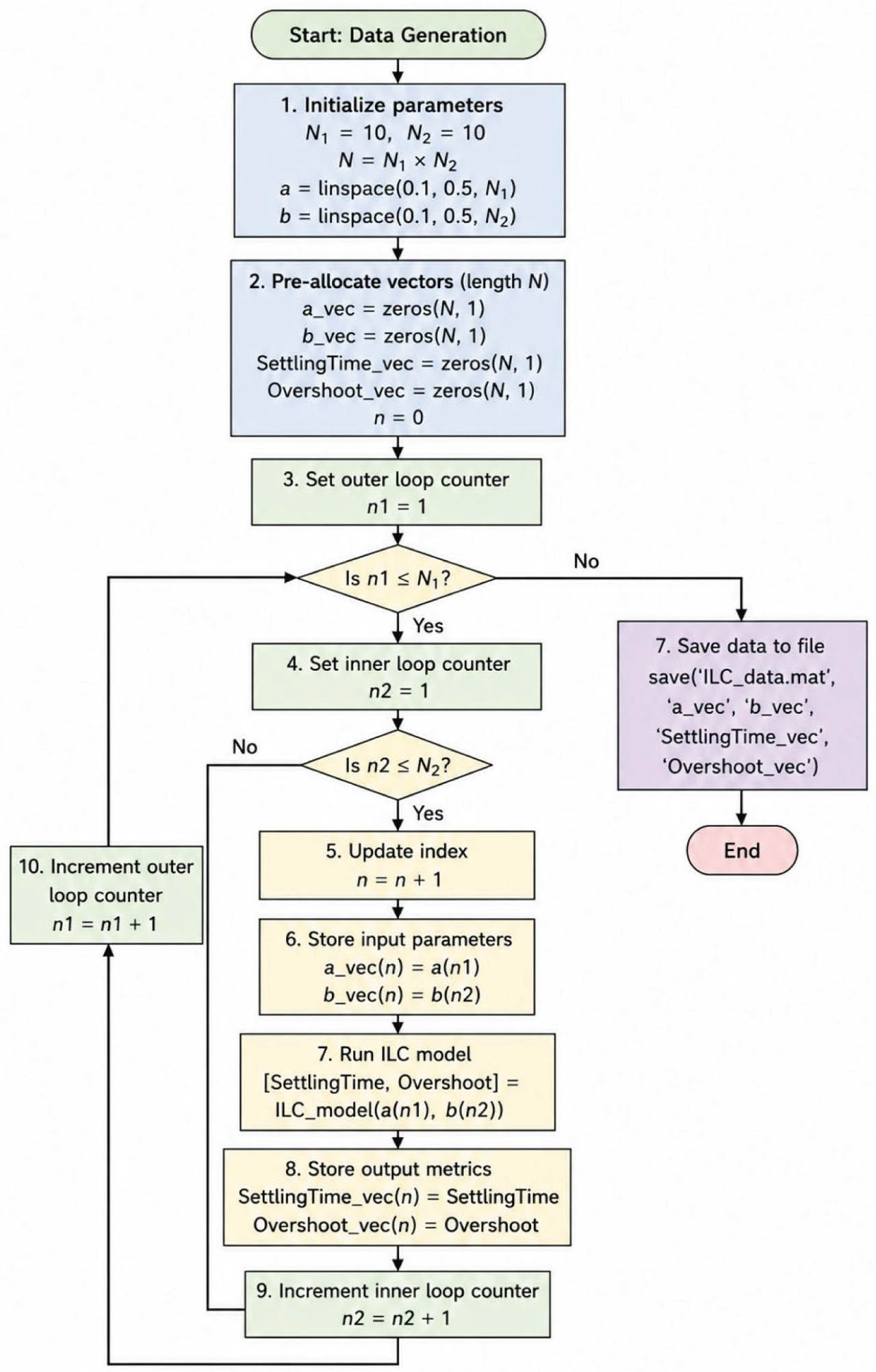
Figure 5.
Flowchart for generating the dataset using MATLAB. ILC, iterative learning control.
5.3. Determination of the optimal network architecture
The optimal architecture of the BNN was found by varying the number of hidden nodes and assessing the log evidence values using Eq. (37). Larger log evidence implies a better trade-off between model accuracy and complexity, i.e. a small risk of overfitting. Figure 6 show the log evidence versus the number of hidden nodes in BNN. As the number of hidden nodes changes, the log evidence increases initially, indicating an improvement in the network’s ability to model the non-linear relationship in the dataset. But at some point, the evidence in the logs starts to fall off as the model gets more complex. The BNN with two hidden nodes has the highest log evidence among all the tested configurations, implying that this structure offers the best trade-off between learning capability and generalisation performance. Hence, BNN architecture with two hidden nodes was selected for the proposed system.
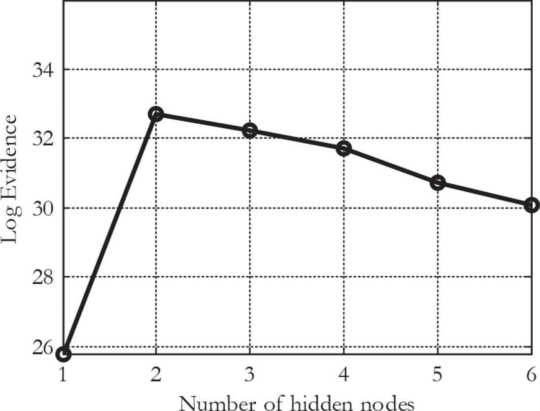
Figure 6.
Log evidence versus number of hidden nodes.
5.4. Network training
After the data generation process, the best values of hyperparameters were found by means of network regularisation. During this phase, the neural network was trained to minimise the cost function and improve the generalisation capability of the model. The model regularisation process controls the complexity of network weights, avoids overfitting and keeps good prediction accuracy. In this study, the training process was performed using the scaled conjugate gradient (SCG) optimisation method (Bishop, 1995) that ensures an efficient and stable convergence during the learning of neural networks. The SCG algorithm iteratively updates the network weights and biases to obtain the minimum value of the cost function with reduced computational complexity and faster convergence than the conventional gradient descent methods.
The BNN training procedure includes the following steps:
Step 1: Initialise the values for α and β. The network weights and biases are initialised from the prior distribution defined for α.
Step 2: Update the vector of weights and biases to minimise the cost function, S (w), using the SCG optimisation method.
Step 3: When the cost function has reached a local minimum, the values of and can be re-estimated as follows:
Step 4: Repeat Steps 2 and 3 until convergence has reached.
The changes of hyperparameters in five re-estimation periods during the training process are shown in Table 2. The value of α increases gradually and the value of β decreases during the re-estimation procedure. These hyperparameters are important for controlling the trade-off between model complexity and data fitting in the Bayesian learning paradigm. The increase in α shows that the regularisation effect on network weights and biases becomes more powerful as the training continues. The penalty term in the cost function, on the other hand, penalises large parameter values, resulting in a smoother and more stable model. The decrease in β also reflects the correction of the data error term during the estimation process. This adaptive modification of the hyperparameters enables the model to reach an adequate trade-off between the minimisation of the training error and good generalisation performance. Thus, the Bayesian training process can effectively prevent overfitting, decrease the sensitivity to noise in the training data and enhance the robustness and predictive capability of the model when it is applied to unseen data. Thus, the re-estimation of the hyperparameters is an important step to improve the overall reliability and generalisation capability of the neural network model.
Table 2.
Changes of the hyperparameters according to five re-estimation periods.
| Re-estimation period | α | β |
|---|---|---|
| 1 | 0.06818 | 154.24078 |
| 2 | 0.09396 | 152.98557 |
| 3 | 0.15781 | 150.32572 |
| 4 | 0.37790 | 147.54382 |
| 5 | 0.45917 | 146.92314 |
Figure 7 illustrates the principle of determining the gains of the ILC controller using a trained BNN. In this approach, the minimum values of the settling time and overshoot vectors are used as the input features of the network. The trained BNN learns the non-linear relationship between the dynamic performance indices and the corresponding optimal controller gains. Based on the input data, the network predicts the appropriate gains of the ILC controller to achieve improved transient response and tracking performance.
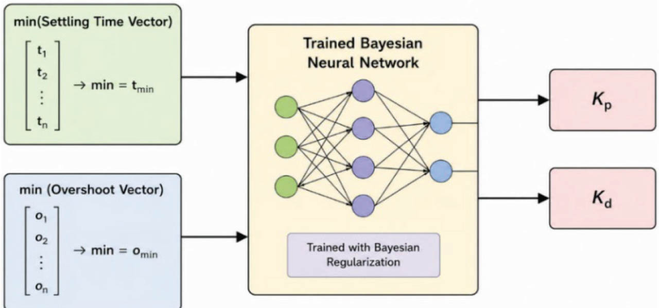
Figure 7.
Principle of determining the gains of the ILC controller using a trained BNN. BNN, Bayesian neural networks; ILC, iterative learning control.
5.5. Simulation
Figure 8 illustrates the flowchart of the simulation of DC gear motor control using a PD-type ILC. Figures 9a,b show the simulated motor speed responses to reference speeds of 500 rpm and 900 rpm, respectively. In both cases, the proposed PD-type ILC controller enables the motor speed to rise rapidly towards the desired reference, demonstrating a fast transient response. Only a slight overshoot is observed before the speed converges to the reference value, indicating that the controller is appropriately tuned and provides an effective balance between response speed and stability. Furthermore, the transient response is well damped, allowing the motor speed to settle quickly with negligible oscillation.
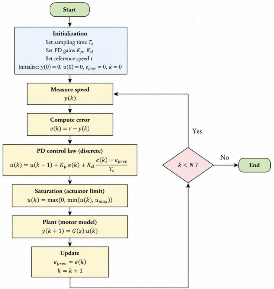
Figure 8.
Flowchart of the simulation of DC gear motor control using a PD-type ILC. ILC, iterative learning control; PD, proportional-derivative.
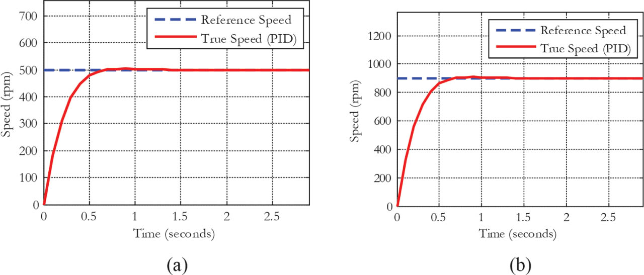
Figure 9.
Simulated motor speed responses to reference speeds of 500 rpm (a) and 900 rpm (b).
Once the transient period has elapsed, the motor speed accurately follows the reference speed with virtually zero steady-state error. The absence of sustained oscillations and the rapid convergence to the desired operating point confirm the stability of the closed-loop system. These simulation results demonstrate that the proposed PD-type ILC controller provides excellent tracking performance over different operating speeds, achieving fast response, minimal overshoot, short settling time and high steady-state accuracy.
5.6. Controller implementation
Figure 10a shows the flowchart for the implementation of the PI controller on the Arduino Nano platform. The flowchart presents the main computational procedures of the controller. The initialisation process, sensor signal acquisition, calculation of the control error, execution of the PI control algorithm, generation of PWM signal and update of the control variables during each sampling interval. The implemented algorithm enables the Arduino Nano to control the motor speed in real time in accordance with the desired reference signal.
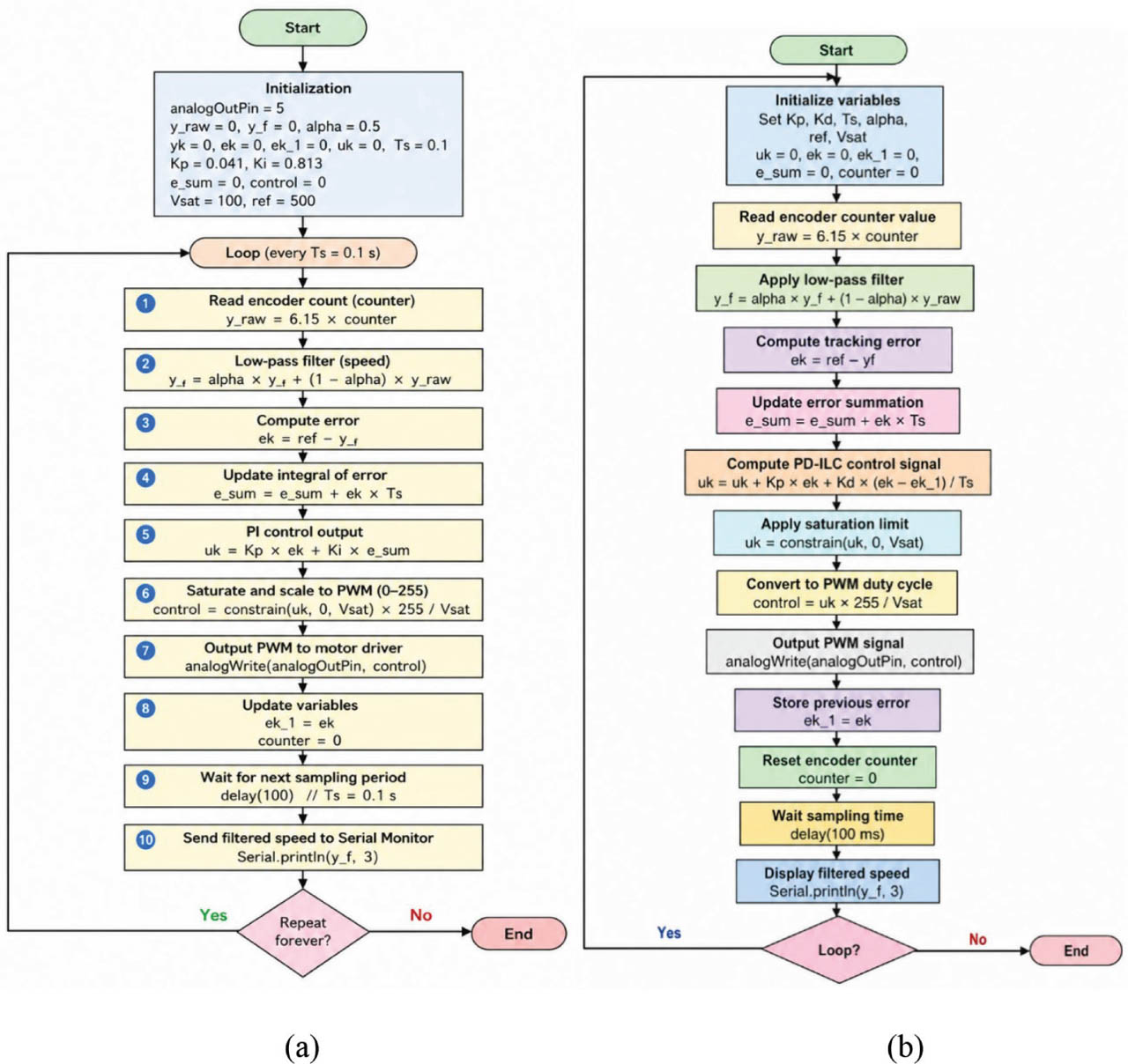
Figure 10.
Flowcharts for implementing the PID controller (a) and the ILC controller (b) on the Arduino Nano. ILC, iterative learning control; PD, proportional-derivative; PI, proportional-integral; PWM, pulse-width modulation.
Figure 10b presents the flowchart for implementing the ILC controller, which is based on an iterative learning process in which the control input is updated at each iteration using the tracking error from the previous iteration. The ILC controller can be used for reducing the steady state error of the system and improving the tracking performance by using repetitive learning cycles. The flowchart also shows the flow of error calculation, learning gain updating, controlling signal generation and iteration management. The flowchart shows how the controller arrives at increasing better performance in each repetition.
Figure 11 shows the block diagram of the proposed closed-loop DP-type ILC speed control system for the DC gear motor. The reference speed is compared with the measured motor speed to produce the tracking error. This error is processed by the ILC controller, which generates the PWM duty cycle for the DC chopper. The DC chopper regulates the armature voltage supplied to the motor, thereby controlling its speed. The encoder measures the motor speed and feeds it back to the controller, forming a negative-feedback loop that minimises the tracking error and ensures accurate and stable speed regulation.
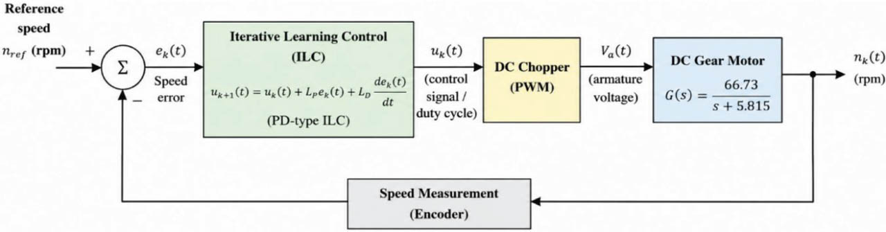
Figure 11.
Block diagram of the ILC-based DC gear motor control system. ILC, iterative learning control; PD, proportional-derivative; PWM, pulse-width modulation.
5.7. Experimental results
Table 3 contains the optimal gains of the trained BNN-based ILC (BNN-ILC) controller. The controller gains were obtained based on the minimum value of the settling time vector and the minimum value of the overshoot vector obtained by the data generation and optimisation procedures. In this method, many operating condition and controller parameter combinations were evaluated to determine the control gains that give the best transient response characteristics for the DC gear motor system. The trained BNN was used to learn the non-linear relation between the system performance indices and the corresponding ILC controller gains. The trained BNN was used to predict optimal control parameters that can provide fast response time with stable system operation, by using the minimum time of settling and overshoot as the optimisation criteria. The gains obtained are thus the best trade-off between fast convergence and low transient oscillation.
Table 3.
The gains of the ILC controller obtained using the minimum values of the settling time and overshoot vectors with a trained BNN.
| Min(settling time vector) | Min(overshoot vector) | KP, ILC | KD, ILC |
|---|---|---|---|
| 0.4625 (s) | 0 (%) | 0.037 | 0.003 |
The proposed PD-type ILC algorithm updates the control input iteratively by utilising information obtained from previous executions of the same repetitive task. Unlike conventional feedback controllers, which generate the control signal solely from the current tracking error, the proposed ILC strategy incorporates the control experience accumulated over successive iterations. Specifically, the control input from the previous iteration is retained and refined by adding a correction term proportional to the current tracking error and its derivative. The proportional component reduces the instantaneous tracking error, while the derivative component predicts the error trend and suppresses oscillatory behaviour, thereby improving the transient response and system stability.
By repeatedly updating the control input in this manner, the controller progressively learns the feedforward control action required to compensate for the motor dynamics and repetitive disturbances. Consequently, the tracking error decreases from one iteration to the next, leading to continuous improvement in tracking performance. Under the convergence condition of the learning algorithm, the control input converges to an optimal profile that enables the motor speed to closely follow the desired reference trajectory. As a result, the proposed PD-type ILC achieves faster convergence, reduced overshoot, shorter settling time and improved steady-state tracking accuracy compared with conventional feedback control methods, making it well suited for repetitive motion and precision speed control applications.
In experimental, the responses of the true motor speed to reference speeds of 500 rpm and 900 rpm are presented in Figures 12a,b, respectively. The experimental results demonstrate that the proposed BNN-ILC controller provides a faster and smoother transient response than the conventional PI controller under both operating conditions. In particular, the proposed controller exhibits significantly reduced oscillations, lower overshoot and improved tracking performance during the transient period. As a result, the motor reaches the desired reference speed more rapidly while maintaining greater stability.
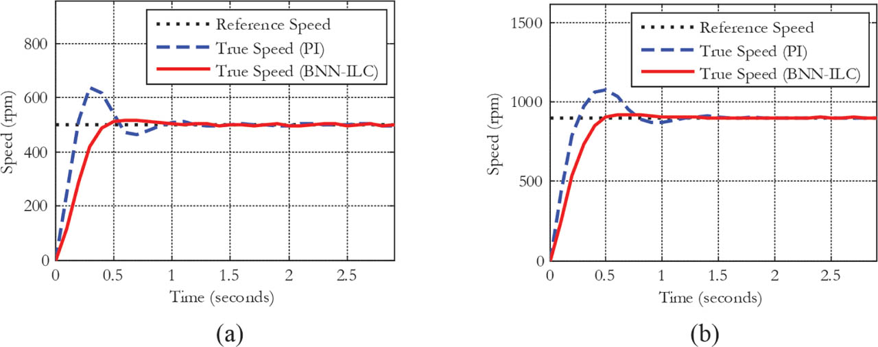
Figure 12.
True motor speed responses to reference speeds of 500 rpm (a) and 900 rpm (b). BNN, Bayesian neural networks; BNN-ILC, BNN-based ILC; ILC, iterative learning control; PI, proportional-integral.
A quantitative comparison of the performance indices is provided in Table 4. The results indicate that the proposed BNN-ILC controller achieves a shorter settling time and lower overshoot than the conventional PI controller. Furthermore, the steady-state tracking accuracy is improved owing to the iterative learning mechanism, which continuously refines the control input based on the tracking error from previous iterations. These improvements confirm the effectiveness of the proposed BNN-ILC strategy in enhancing both the dynamic response and tracking accuracy of the DC gear motor. The consistent performance observed at both 500 rpm and 900 rpm also demonstrates the robustness of the proposed controller under different operating conditions, making it a promising approach for high-performance motor speed control applications.
6. Conclusions
An efficient data-driven method to tune the parameters of a PD-type ILC system for DC gear motors is this study. The BNN was designed to predict the optimal controller gains with uncertainty quantification to improve the robustness, reliability and generalisation capability of the tuning process. An approximate mathematical model of the DC gear motor was used to generate a dataset under different operating conditions to train the BNN to estimate the optimal control gains that minimise the tracking errors that occur in the iterative learning process. The experimental results demonstrate that the proposed BNN-based ILC scheme exhibits faster convergence, shorter settling time and lower overshoot than the conventional PI controller, and possesses better adaptability to various operating conditions. The BNN’s probabilistic nature allows the approach to deal with the uncertainty of the tuning process. The proposed method is also capable of optimising diverse kinds of controllers, like PID controllers. The same data-driven framework and BNN approach can determine the optimal controller parameters under different operating conditions to improve the system performance. Furthermore, the suggested approach can be extended to other advanced control techniques, offering better robustness, adaptability and tracking precision in a large variety of control applications.
Acknowledgements
This research is funded by Hanoi University of Science and Technology (HUST) under project number T2025-PC-083.