
1. Introduction
As decentralised energy flows become more complicated, artificial intelligence (AI) algorithms are becoming crucial for smart microgrids to increase the use of renewable energy and maintain stability during changes in demand. From a technical standpoint, the implementation of AI algorithms makes it possible to establish multidimensional management of microgrids (Talaat et al., 2023), aiming to reconcile the optimisation of operational costs with technical imperatives such as power smoothing, rigorous control of the state of charge (SOC) of batteries and peak shaving (Reihani and Sepasian, 2016).
The operational implementation of these regulations and optimisation functions requires the harmonious integration of the physical components of the smart grid, namely generators such as photovoltaic panels (PV), wind turbines, and fuel, as well as storage devices (Khan et al., 2024). The diversity of smart microgrid infrastructure also impacts the performance of AI control and the battery management system (BMS).
The dependence on an already fragile electricity grid, combined with the abundance of largely untapped renewable resources, highlights the need to adopt decentralised energy solutions capable of strengthening local resilience. In this context, the concept of the smart microgrid appears as a particularly suitable approach, enabling the integration of photovoltaic production, wind power, and storage to respond autonomously and flexibly to fluctuations in demand (Lamia and Adnen, 2023). However, the efficiency of a microgrid relies heavily on its ability to intelligently combine these different sources and optimise energy flows in real time. This is why the integration of AI techniques into management mechanisms, particularly through intelligent controllers for batteries and conversion systems, represents a key lever for improving the stability, efficiency, and sustainability of the local energy system (Thirunavukkarasu and Sawle, 2021).
1.1. Related work
In recent years, several studies have explored the integration of photovoltaic, wind, and storage systems within smart microgrid architectures, proposing intelligent control methods to improve BMS and enhance system resilience. Authors in Soliman et al. (2021) introduce a compact energy management EMS strategy for a smart DC microgrid based on a hybrid fuzzy logic controller (FLC)–high-order sliding mode (HSMC) controller. The system integrates a battery bank with wind, PV, and tidal sources. The proposed controller maximises renewable energy extraction, enhances DC microgrid power quality, and prioritises low-cost renewable generation while ensuring stable and reliable operation. Albarakati et al. (2021) present an EMS for a hybrid microgrid integrating solar, wind, Li-ion storage, and grid backup. Renewable sources operate under maximum power point tracking (MPPT) via a Multi-Agent System, while battery charging and discharging are optimised using artificial neural network (ANN) controllers. The system ensures power balance and flexible adaptation to varying operating conditions, with implementation carried out in MATLAB/Simulink and JADE through MACSIMJX.
Deep learning also contributes to optimising smart microgrids, as in Lami et al. (2025), a deep reinforcement learning (DRL) and ANN-based platform for real-time energy optimisation, demand forecasting, and peer-to-peer (P2P) trading. The system reduces energy costs by 23%, lowers grid dependence by 40%, and achieves 85% renewable penetration. The applicability of the proposed V2H strategy remains limited for households that do not own electric vehicles, highlighting the need for alternative energy storage solutions to ensure broader adoption. Meanwhile, authors in Moazzen and Hossain (2024) focus on forecasting by evaluating a multivariate machine learning forecasting framework for microgrid EMSs using multiple long short-term memory neural networks (LSTM) architectures. This multivariate forecasting approach shows that it may lead to lower prediction accuracy compared to simpler univariate models due to the additional complexity and noise introduced into the learning process; besides, the results demonstrate that low forecasting errors do not necessarily guarantee near-optimal economic performance. In Sun et al. (2025), a two-stage robust optimisation framework is proposed using bidirectional temporal convolutional networks (BiTCN)–Transformer forecasting, achieving high accuracy (MAE 1.3512, R2 0.9683). Simulation under high and low wind scenarios shows improved renewable utilisation, reduced emissions, and enhanced reliability. However, the uncertainty modelling and deep learning framework in this study focus exclusively on wind energy generation, while other renewable energy sources, particularly photovoltaic systems, are not considered, and the proposed strategy relies on a centralised offline robust optimisation approach based on the C&CG algorithm, which may limit its adaptability to real-time BMS applications.
Table 1 summarises the previous works discussed in this section.
Table 1.
Literature review.
| Reference | Microgrid energy sources | Method | Objective | Real-world data | Comparative study | Economic analysis |
|---|---|---|---|---|---|---|
| Soliman et al. (2021) | PV + wind + tidal sources + battery | FSHSMC is a combined FLC and HSMC | Energy management control technique for a smart DC-microgrid | × | ✓ | × |
| Albarakati et al. (2021) | PV + wind + battery | MPPT + multi-agent system MAS | Maintain the power balance in the microgrid | × | ✓ | × |
| Lami et al. (2025) | PV + wind + battery | DRL and neural networks | Real-time energy optimisation, demand forecasting, and P2P trading optimise energy consumption, predict demand, and facilitate P2P energy trading. | ✓ | ✓ | ✓ |
| Moazzen and Hossain (2024) | PV + wind + battery + grid | LSTMs | Optimise distribution, reduce grid dependence, and maximise renewables | ✓ | ✓ | ✓ |
| Sun et al. (2025) | Wind + heat + gas + hydrogen | BiTCN | Minimise the overall operational cost, including transaction costs, fuel costs, and maintenance expenses. Improving renewable energy utilisation and system reliability | ✓ | × | ✓ |
1.2. Scientific contributions
Although AI algorithms are increasingly integrated into smart microgrid BMSs, several limitations remain poorly understood. Recent literature focuses primarily on highly complex deep learning forecasting models or optimisation-centric architectures, which require large datasets, significant computing resources, and advanced training procedures. Furthermore, the dynamic behaviour of conventional smart controllers under unstable grid operating conditions remains insufficiently analysed, particularly during short-duration transient regimes involving battery demand and fluctuations in renewable energy production.
To address these limitations, this work proposes and evaluates two intelligent BMS strategies based on fuzzy logic (FL) control and ANN within a hybrid smart microgrid integrating photovoltaic generation, wind energy, battery storage, residential loads, and grid interaction. The proposed strategies are estimated under varying load demand conditions, including periods of increased power consumption when the grid alone may be unable to satisfy the total energy requirements, thereby requiring effective battery support.
The main contributions can be outlined as follows:
- Development of a comparative framework for FL and ANN under identical operating conditions.
- Performance evaluation during a peak load stress scenario leading to grid instability.
- Integration of real meteorological measurements from the Gafsa region (Tunisia), allowing realistic evaluation of the proposed smart microgrid under actual climatic conditions.
- Economic analysis showing the impact of intelligent BMS on operational energy costs and battery utilisation efficiency.
1.3. Study organisation
The remainder of this paper is organised as follows. Section 2 presents the modelling framework of the proposed smart microgrid architecture. Section 3 details the implementation of AI-based strategies for battery management control: FL and ANN. Section 4 evaluates and compares the performance of the system controlled by FL and ANN using real climatic measurements from Gafsa region. In section 5, a detailed economic analysis is conducted to quantify the efficiency gains under real meteorological data. Finally, Section 6 summarises the main findings of the paper and outlines potential directions for future research.
2. Smart Microgrid Architecture and Modelling
2.1. Smart microgrid system description
The studied microgrid system is a smart, decentralised energy system that integrates various sources of energy production, storage, and consumption within a local grid capable of operating in a grid-connected or stand-alone mode (Arévalo et al., 2025; Shahgholian, 2021). In the configuration studied and presented in Figure 1, the microgrid includes a wind turbine, a photovoltaic generator, a battery storage system, the main grid, and a domestic load. The wind turbine converts the kinetic energy of the wind into electricity, while the photovoltaic panels harness solar energy to produce continuous power dependent on irradiance and temperature. These renewable sources, characterised by their variability, are coupled with power converters ensuring regulation and synchronisation with the microgrid’s common bus.
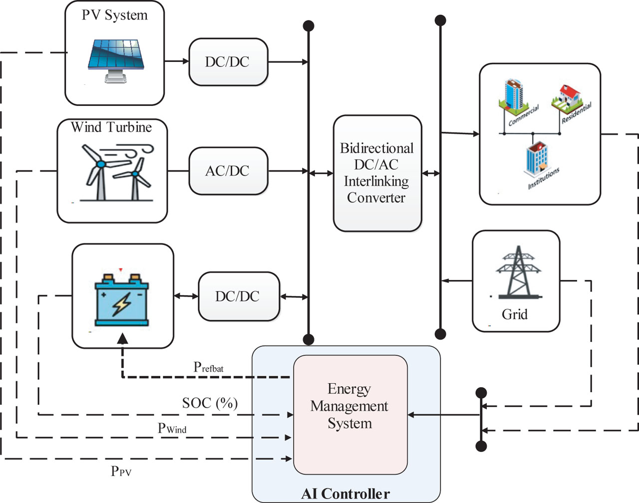
Figure 1.
Smart microgrid system with AI-based controller. AI, artificial intelligence; SOC, state of charge.
The storage system plays a crucial role in stabilising the local network, absorbing excess production and restoring energy during periods of deficit, thanks to a bidirectional converter allowing energy exchanges between the battery and the grid (charge and discharge modes). The microgrid can also exchange energy with the main grid, either to import power in case of local insufficiency or to inject surplus production, thus improving the flexibility and reliability of the system. The generated energy is finally distributed to the residential load, representing the electrical demand of homes. The BMS supervises the battery status and regulates charging and discharging operations based on the battery’s condition and energy availability to ensure a dynamic balance between production, storage, and consumption while maximising the energy efficiency and sustainability of the microgrid.
2.2. Smart microgrid component model
2.2.1. Solar energy system
The solar energy subsystem is modelled using a photovoltaic generator PV that converts incident solar irradiance into electrical power according to the non-linear current–voltage characteristics of the PV cells. This phenomenon is based on the interaction between photons and a semiconductor material, generally silicon-based, forming a PN junction. When a photon of the appropriate energy reaches this junction, it can excite an electron, causing a bond to break and creating an electron–hole pair. The internal electric field of the junction separates and sets these charges in motion, thereby generating a usable electric current (Ouammi, 2021). Figure 2 shows a common electrical model of a solar cell (Batzelis, and Papathanassiou, 2015).
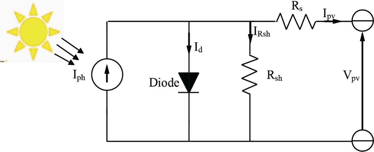
Figure 2.
The equivalent electrical circuit of photovoltaic (PV).
The current generated by the cell is expressed by the following expression:
Where:
Iph : light-generated current (A),
Is : diode saturation current (A),
VPV: the cell voltage (V),
Rs, Rsh : series and shunt resistance (Ω),
α: diode ideality factor and
VT : Thermal voltage (V).
And the thermal voltage is presented by:
Where:
n : Number of series-connected cells,
K : Boltzmann constant (1.380649 × 10⁻²³ J/K) and
T : Absolute temperature (K) and
q : Electron charge (1.602176634 × 10⁻⁹ C)
The MPPT is a control strategy widely used in photovoltaic systems to continuously adjust the operating point of the solar panel so that it delivers the maximum possible power under varying environmental conditions. In fact, the MPPT control principle ensures that the PV system always operates at the optimal point by controlling the duty cycle of the DC/DC converter depending on the current voltage, power voltage, solar irradiance, and temperature (El Hammoumi et al., 2022).
In this study, the photovoltaic system is configured using photovoltaic modules arranged in 37 parallel strings and 6 series-connected modules per string, providing an installed capacity of approximately 40 kW. Each module is composed of 60 interconnected solar cells. The electrical characteristics of the adopted PV module are summarised in Table 2.
Table 2.
PV module parameters.
| Parameter | Value |
|---|---|
| Light-generated current | 10.0926 A |
| Diode saturation current | 3.323 × 10⁻¹¹ A |
| Shunt resistance | 212.8143 Ω |
| Series resistances | 0.31448 Ω |
| Maximum power | 302.2 W |
| Cell per module | 60 |
| Short-circuit current | 10.05 A |
| Open circuit voltage | 32.5V |
The PV model parameters were intentionally designed to be representative of a realistic photovoltaic generation system while satisfying the energy demand of the studied microgrid. Particular attention was given to maximising the exploitation of the available solar resource in the considered case study. Correspondingly, the parameters of the single-diode equivalent model, including the series resistance Rs and shunt resistance Rsh, were automatically identified by the MATLAB/Simulink PV Array model from the specified electrical characteristics of the customised module to accurately reproduce its I–V and P–V behaviour.
2.2.2. Wind energy system
The wind energy system consists of a 10 kW variable-speed wind turbine coupled to a permanent magnet synchronous generator (PMSG) to convert the mechanical power extracted from the turbine into electrical power with high efficiency and stable dynamic behaviour (Gaied et al., 2022; Majout et al., 2022). The PMSG is modelled using the standard non-linear electromechanical equations expressed in the dq-rotor reference frame, which allow an accurate description of the stator flux, electromagnetic torque, and rotor dynamics (Prince et al., 2021). The stator voltage equations are given by:
Where Rs is the stator resistance, ωe the electrical angular speed, and λd, λq the flux linkages are defined as:
With Ld and Lq denoting the stator inductances and λm the permanent magnet flux. The electromagnetic torque is expressed as:
With p being the number of pole pairs.
The rotor mechanical dynamics are modelled by:
Where J is the rotor inertia, B the viscous friction coefficient, Tm the mechanical torque supplied by the wind turbine, and ωm the mechanical speed.
Finally, the aerodynamic wind power is presented by Eqs (8) and (12)
Where ρ: Air density, A = πR2 : Surface swept by the rotor, Cp(λ, β) : power coefficient dependent on tip speed ratio and pitch angle, vm : wind speed and : tip speed ratio.
To ensure optimal energy extraction from the wind, the generator also operates under an MPPT strategy. The MPPT algorithm continuously adjusts the electrical torque imposed on the PMSG, typically by manipulating the duty cycle of the AC/DC converter to regulate the generator speed so that it matches the optimal tip-speed ratio corresponding to maximum aerodynamic efficiency. By dynamically shaping the electrical load seen by the generator, the MPPT maintains operation on the turbine’s maximum power curve despite rapid variations in wind speed. This coordinated electromechanical modelling therefore captures the full coupling between turbine aerodynamics, PMSG dynamics, and converter-level MPPT control, providing a realistic foundation for performance assessment within the smart microgrid (Bakbak et al., 2022).
The considered model is representative of small-scale distributed wind energy conversion systems that ensure compatibility with the power requirements of the proposed smart microgrid. The main electrical and mechanical characteristics of the PMSG model and the wind turbine used in this study are presented in Table 3.
Table 3.
PMSG and wind turbine electrical and mechanical parameters.
| Parameter | Value |
|---|---|
| Number of pole pairs | 4 pairs |
| Permanent magnet flux linkage | 0.1688 Wb |
| Stator Resistance Rs | 0.0918 Ω |
| Rotor Inertia J | 0.003945 Kg m2 |
| Viscous damping coefficient B | 0.0004924 N m s |
| Back-EMF waveform | Sinusoidal |
| Rotor type | Round |
| Rated mechanical power | 10 KW |
| Rated wind speed | 12 m/s |
| Maximum power coefficient | 0.48 |
2.2.3. Lithium-ion battery energy storage system
The energy storage subsystem is implemented using a lithium-ion battery, which can be represented by an equivalent electrical circuit composed of an open-circuit voltage source UOCV(SOC) and an internal resistance Rint(SOC). The equivalent circuit is illustrated in Figure 3 (He et al., 2011; Islam et al., 2020).
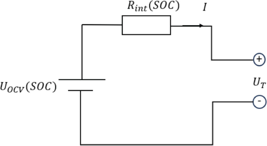
Figure 3.
Lithium-ion equivalent circuit model. SOC, state of charge.
Unlike conventional battery models, where these parameters are assumed to be constant, both the open-circuit voltage UOCV(SOC) and Rint(SOC) depend on the battery’s SOC. The open-circuit voltage increases with the SOC according to the battery’s open-circuit voltage characteristic, while Rint(SOC) varies with the operating condition of the battery and is generally higher at low and high SOC levels, reaching its minimum value in the intermediate SOC range. Consequently, the battery terminal voltage can be expressed as:
Where, I denotes the battery current being positive during discharging and negative during charging.
The SOC evolution is determined using the Coulomb counting method, which estimates the remaining charge by integrating the battery current over time:
Where Qnom is the nominal capacity.
The technical specifications of the battery model used in our work are summarised in Table 4.
2.2.4. Grid and residential load
In the proposed smart microgrid model, the electrical grid is represented as a stable three-phase voltage source (400V, 50 Hz) that serves as a power reference and is often modelled by the following equation (Espín-Sarzosa et al., 2024; Nair et al., 2022):
The coupling between the microgrid and the network is ensured via a bidirectional inverter, the exchanged power of which is the following:
For the residential load, it is modelled as a time-varying electrical demand reflecting typical household consumption patterns. It is implemented as a dynamic load block connected to the AC bus, imposing an instantaneous power demand depending on the active power. Pload and the reactive power Qload expressed respectively by the following equation:
3. Smart Control Strategies for BMSs
3.1. Battery management strategy
The lithium-ion battery in the proposed smart microgrid is governed by an intelligent BMS designed to ensure optimal operation, protect battery health, and maintain power balance within the system. The BMS receives real-time measurements of battery current, terminal voltage, and SOC and determines the appropriate charging or discharging action according to the instantaneous conditions of the microgrid (Garjola et al., 2025).
To enhance decision-making accuracy under non-linear and uncertain operating environments, two AI-based controllers, FL and ANN are implemented and compared. These controllers regulate the bidirectional power converter interfacing the battery with the DC bus, thereby determining the direction and magnitude of the energy flow (Madani et al., 2025).
Figure 4 represents a block diagram of the AI-based BMS. It is underlined that the real-time measurements of PV and wind power, DC bus voltage, and battery variables (SOC, current and voltage) are used as inputs to the intelligent controller. Depending on the selected method FL or ANN, the BMS generates the optimal charging or discharging command for the bidirectional DC/DC converter to regulate the energy flow of the lithium-ion battery.
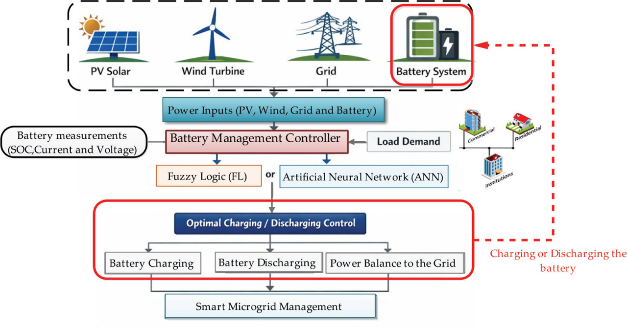
Figure 4.
Block diagram of the AI-based BMS. AI, artificial intelligence; ANN, artificial neural network; BMS, battery management system; FL, fuzzy logic; SOC, state of charge.
3.2. FLC model
The fuzzy controller implemented in this study is of the Mamdani type, a formulation widely adopted in non-linear and uncertain control environments due to its ability to translate human reasoning into a set of linguistically expressed rules (Romdhane et al., 2023).
Figure 5 represents the proposed FL control design.
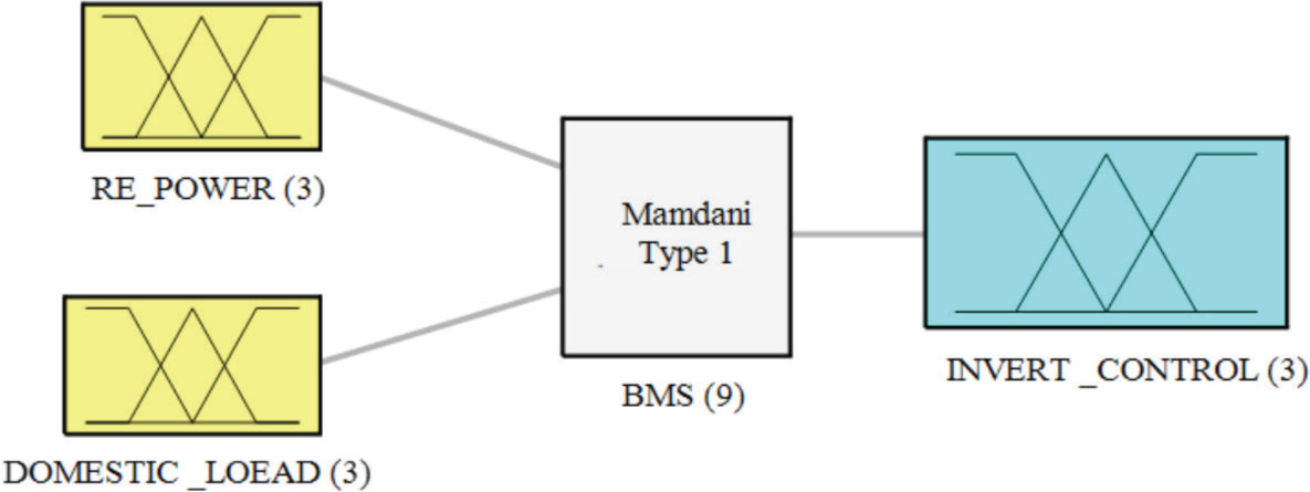
Figure 5.
FL control design. BMS, battery management system; FL, fuzzy logic.
It is designed with two input variables and one output variable, representing the BMS behaviour of the smart microgrid. The input variables correspond to: Renewable energy power availability and Domestic load demand. Figure 6a and 6b depict the input’s membership function. The controller output determines the command applied to the bidirectional inverter, which regulates the charging or discharging process of the lithium-ion battery. The fuzzy partitions include ‘Discharge’, ‘Neutral’ and ‘Charge’, which are presented in Figure 6c.
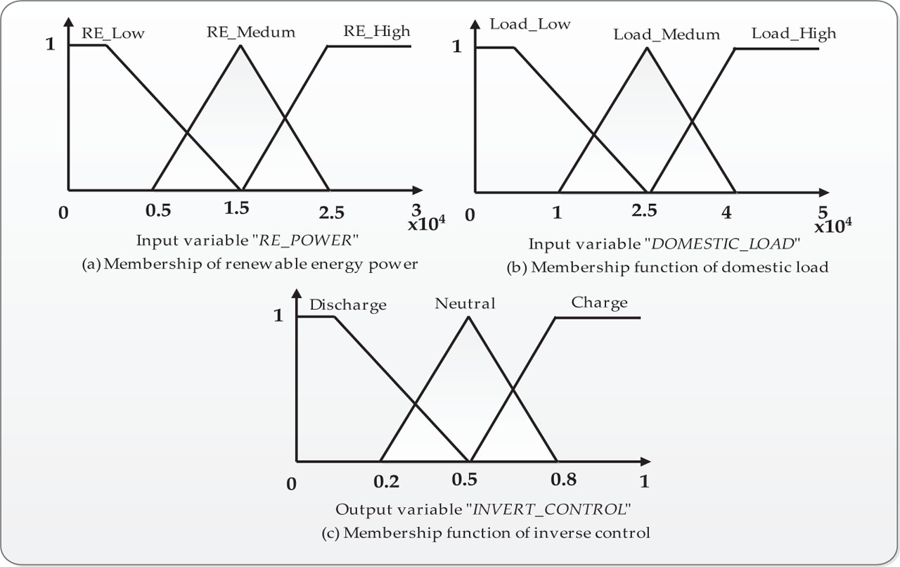
Figure 6.
Distribution of membership functions defined for both the input and output parameters. (a) Membership of renewable energy power. (b) Membership function of domestic load. (c) Membership function of inverse control.
To capture the full operating domain of the microgrid, each input variable is described by three fuzzy membership levels: Low, Medium, and High, leading to a total of nine fuzzy rules that encompass all possible combinations of the input states. The general form of the control rule is expressed as:
If (ER = level x) AND (Load = level y) THEN (Inverter Control = level z)
Where x, y and z denote the linguistic levels assigned to each variable. These rules determine whether the inverter should command battery charging, discharging, or remain in a neutral/steady state. The output variable INVERT_CONTROL is a normalised supervisory command used to determine the operating mode of the battery energy storage system. Depending on its value, the battery is commanded to charge, remain in a neutral state, or discharge through the bidirectional converter.
After the inference stage, defuzzification is performed using the centroid (centre of gravity) method, ensuring a smooth and continuous control signal suitable for real-time operation of the bidirectional inverter.
The complete configuration of the nine fuzzy control rules is presented in Table 5, summarising the connection between renewable energy availability, load demand levels, and the resulting inverter control action.
Table 5.
FL rules configuration.
| Rule | Input 1: Renewable energy power | Input 2: Domestic load demand | Output: Inverter control |
|---|---|---|---|
| 1 | Low | Low | Neutral |
| 2 | Low | Medium | Discharge |
| 3 | Low | High | Discharge |
| 4 | Medium | Low | Charge |
| 5 | Medium | Medium | Neutral |
| 6 | Medium | High | Discharge |
| 7 | High | Low | Charge |
| 8 | High | Medium | Charge |
| 9 | High | High | Neutral |
Figure 7 shows the three-dimensional surface of the proposed FL. This surface provides a visual presentation of the non-linear mapping between the inputs and the output.
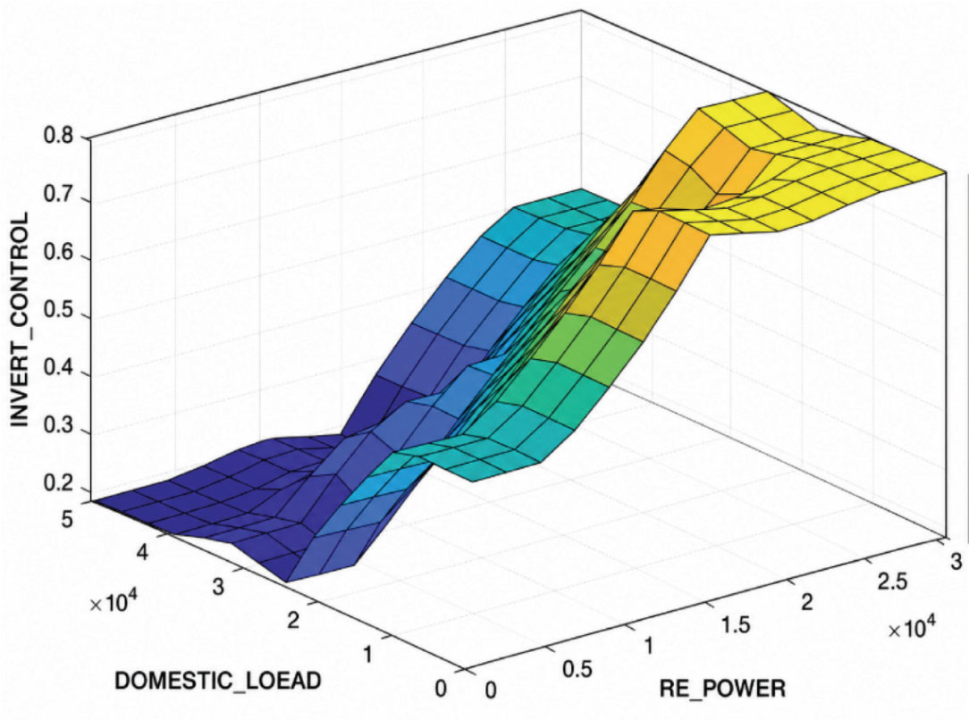
Figure 7.
3D FL surface. FL, fuzzy logic.
3.3. ANN controller model
As the second control algorithm proposed in this study, a compact feedforward ANN is implemented to regulate the battery charging and discharging processes within the smart microgrid. The ANN consists of a single hidden layer with 10 neurones using the logarithmic sigmoid activation function (logsig) and an output layer employing a linear activation function (purelin). The network input corresponds to the energy error, derived from the instantaneous difference between renewable power availability and the charging power required by the microgrid (Abbass et al., 2023; Mariyaraj and Thankappan, 2024). This conversion of the power imbalance into energy error over the sampling interval Δt is defined by:
Where;
The configuration of the layers and the organisation of the neurones constituting the designed ANN model are shown in Figure 8.
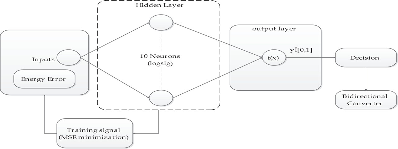
Figure 8.
Proposed ANN architecture. ANN, artificial neural network.
The ANN is trained using the backpropagation algorithm, which iteratively adjusts synaptic weights to minimise the mean squared error between the network output and the desired reference signal. This enables the ANN to approximate the non-linear mapping between the energy imbalance and the optimal battery control action.
Thus, the ANN provides an adaptive control mechanism capable of adjusting the battery charging and discharging processes according to the power exchanged and the microgrid’s energy imbalance. It generates a supervisory decision signal that manages the operating mode of the battery energy storage system and the corresponding control action applied to the bidirectional converter.
The output of the ANN is given by:
Where e : The input error between renewable power and load power, wi1, b1i : The weight and bias of the hidden layer, vi, b2 : The weight and bias of the output layer and s : The signal output.
Although the output layer employs a linear activation function (purelin), the ANN output is constrained to the interval [0,1] through output normalization and saturation. The resulting supervisory signal is defined as:
Where y and ysat represent the ANN output prior to saturation and the bounded control signal used by the BMS, respectively. The normalised output range is divided into three balanced decision regions of equal width to distinguish between the different battery operating modes. Accordingly, the battery operating mode is determined as follows:
This partitioning ensures a clear separation between charging, neutral, and discharging states while maintaining smooth transitions between operating modes.
From Figure 9, the training regression shows a good linearised relation where the general correlation coefficient R = 0.99988 is too close to 1, which reflects the precision of the prediction.
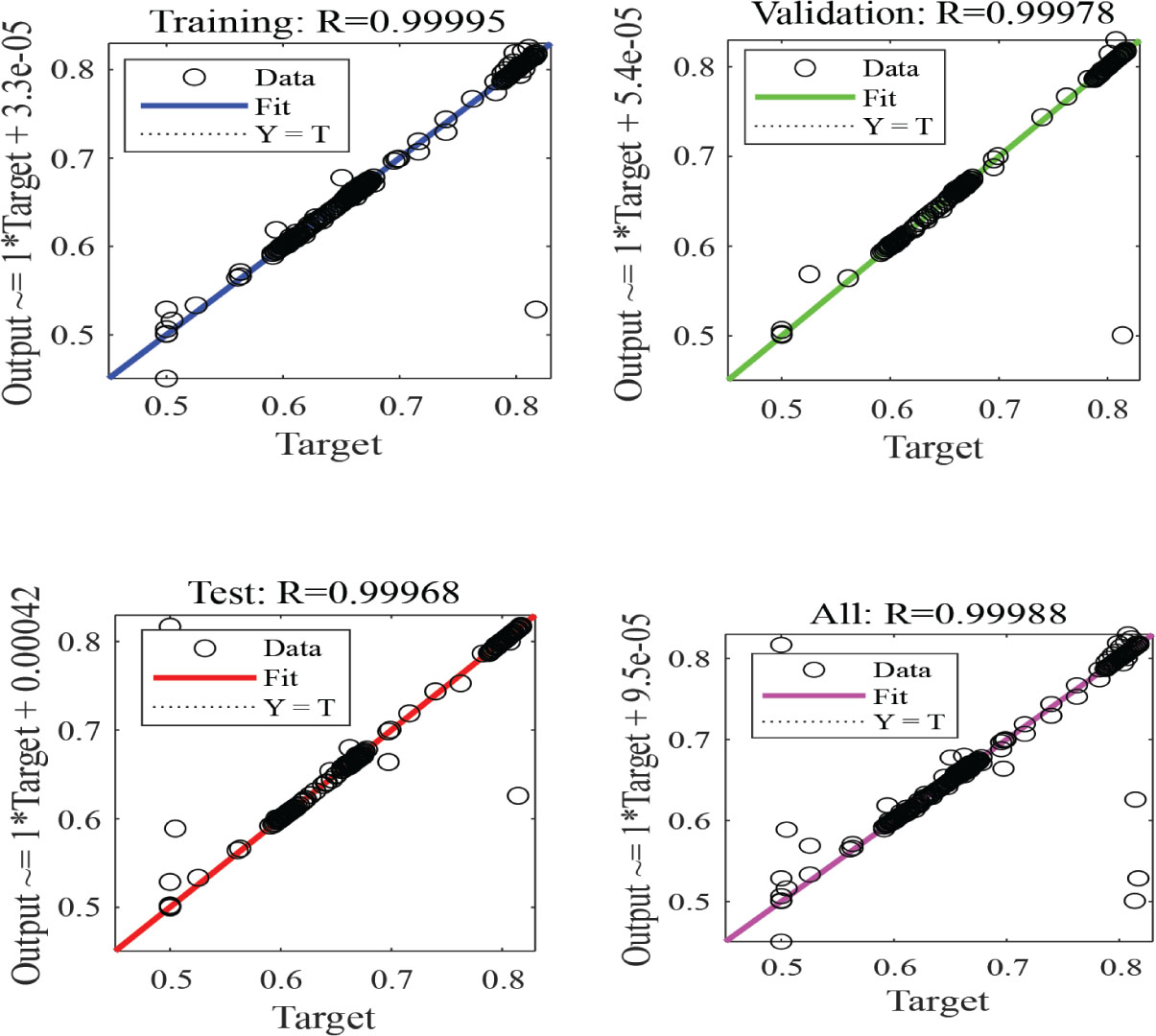
Figure 9.
ANN training regression. ANN, artificial neural network.
The training state in Figure 10 shows that the gradient is 1.264610−5, which is very low, which means the algorithm has converged to the optimal solution; thus, the training is stable. On the other hand, the training step adaptation parameter Mu is 10−8, which is also very low.
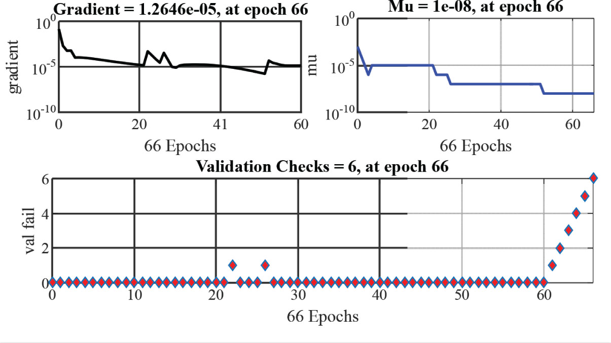
Figure 10.
ANN training state. ANN, artificial neural network.
An early stopping was triggered at epoch 66 when the validation check reached its maximum value of 6, ensuring stable convergence of the ANN.
Figure 11 represents training performance, which shows that the best validation performance by mean squared error is 2.0765110−6 which too small, it is indicates that the network successfully predicts the output.
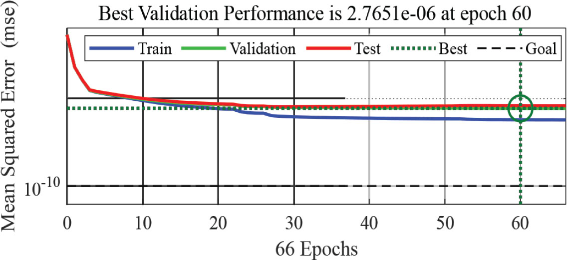
Figure 11.
ANN training performance. ANN, artificial neural network.
Consequently, the ANN converged successfully. The best performance was achieved around the 60th iteration, after which the training process stopped at the 66th iteration due to the absence of further improvement in the validation error. The low gradient value and the minimal value of the damping parameter Mu confirm the stability of the learning process and the successful convergence of the ANN model.
The main parameters of the ANN are summarised in Table 6.
Table 6.
ANN parameters.
| Parameter | Value |
|---|---|
| Input | 1 (energy error) |
| Output | 1 (battery charge/discharge command) |
| Target generation method | Supervised learning based on the desired battery power management response derived from the microgrid energy balance conditions |
| Layer size | 10 |
| Dataset | 2,000 |
| Training algorithm | Backpropagation |
| Training | 70% |
| validation | 15% |
| Test split | 15% |
Figure 12 outlines the main stages involved in designing a neural network-based controller that can be adapted to a wide range of control applications and validated through real-time experimental testing.
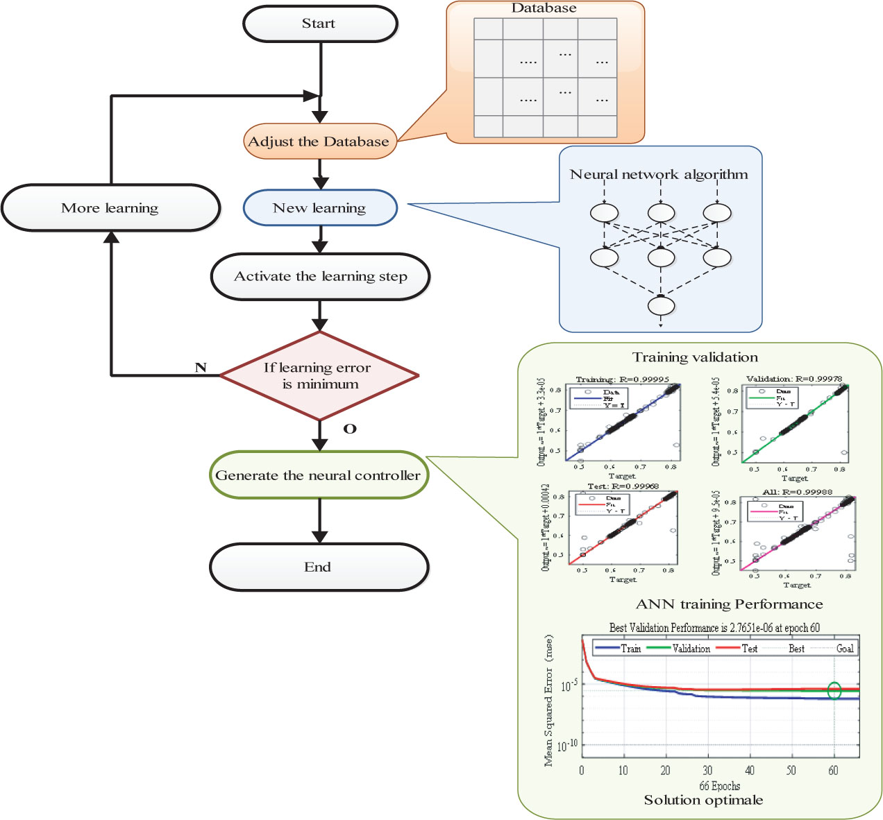
Figure 12.
Key stages involved in developing and deploying a neural network controller.
4. Simulation Results
This section presents and discusses the simulation results obtained for the proposed smart microgrid, which is evaluated under real operating conditions of Gafsa region, with particular emphasis on the comparative performance of the FL and ANN based battery management strategies under different operating conditions.
Table 7 presents the simulation parameters established using the technical data of the PV and wind power systems.
Table 7.
Global system parameters.
| Component | Parameter | Value |
|---|---|---|
| PV system | Power | 40 KW |
| Voltage | 192V | |
| Current | 198.66 A | |
| Number of modules | 222 | |
| Wind system | Power | 10 KW |
| Battery | Voltage | 155V |
| Nominal capacity | 130 Ah | |
| Load | Nominal power | 20 KW |
Figure 13 presents the proposed microgrid implementation architecture developed in the MATLAB/Simulink environment, which constitutes the simulation framework chosen for validating battery management strategies.
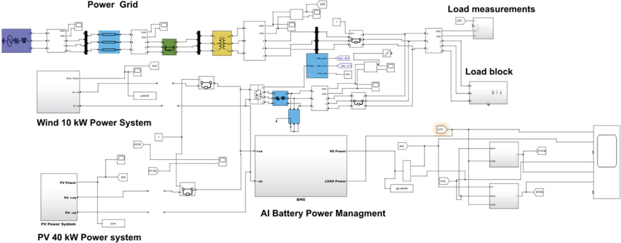
Figure 13.
Global proposed microgrid MATLAB/Simulink model.
4.1. Global system evaluation
Figures 14 and 15 illustrate the dynamic responses of wind and PV power to variations in wind speed and solar irradiance, respectively. As shown in Figure 14a, the wind speed varies stepwise from approximately 8 m/s to 15 m/s over a 2 seconds simulation period. The corresponding wind power response in Figure 14b follows this variation, increasing from about 1.2 × 10⁴ W at low wind speeds to nearly 4 × 10⁴ W at higher velocities and dropping sharply when the wind speed decreases to around 5 m/s.
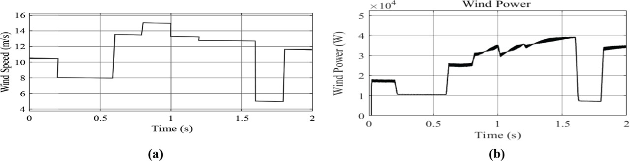
Figure 14.
Wind power for different wind speeds. (a) Wind speed. (b) Wind power.
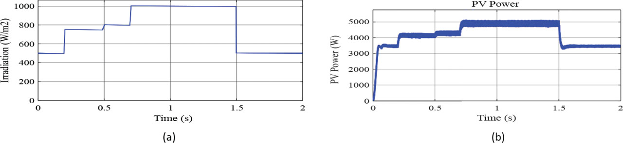
Figure 15.
PV power for different solar irradiance. (a) Solar irradiance. (b) PV power.
Similarly, Figure 15a presents step changes in solar irradiance from 500 W/m2 to 1000 W/m2, followed by a decrease to 500 W/m2. As depicted in Figure 15b, the PV power output rises accordingly from approximately 3.5 kW to about 5 kW at maximum irradiance and decreases to nearly 3.4 kW when it is reduced. These results confirm the strong correlation between renewable resource availability and the generated power.
Over the course of the simulation, Figure 16 shows the power supplied by the photovoltaic (PV) and wind energy systems, their combined output power, the excess generated power, and the load demand. The load is kept constant at 20 kW. As can be seen, the PV system is the main energy source, with the wind turbine providing a lesser but comparatively steady quantity of power. As a result, during the simulation, the total generated power (PV + wind) gradually rises from about 21–43 kW. The findings show that for the majority of operation intervals, the hybrid renewable energy system can meet the load requirement. A power shortfall of roughly 6 kW is needed at the start of the simulation, and another shortage of about 8.5 kW occurs between 1.6 seconds and 1.8 seconds. On the other hand, during the intermediate intervals, especially between 0.6 seconds and 1.6 seconds, a considerable power surplus is produced, with excess power approaching 23 kW. This extra energy can be added to the electric grid or stored in an energy storage system.
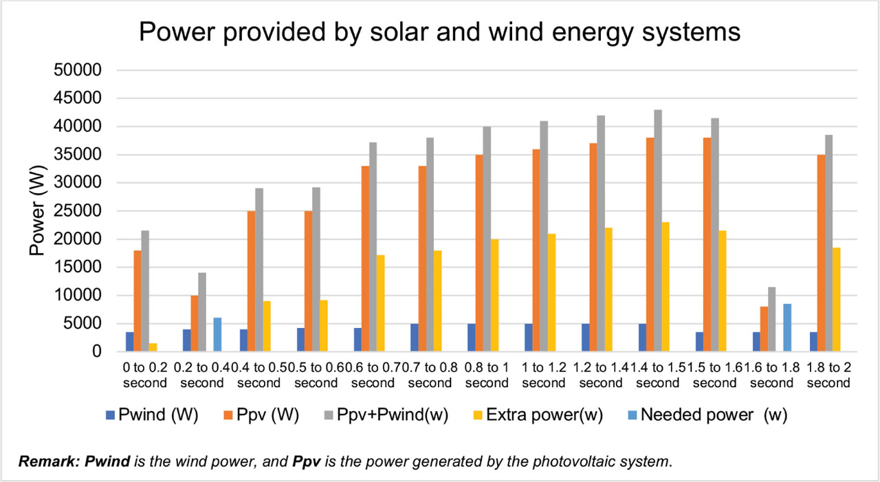
Figure 16.
Power supplied by the PV and wind systems.
Regarding computational complexity, the proposed FL Controller exhibits low computational cost due to its rule-based inference system, involving a fixed set of nine rules and simple defuzzification operations, suggesting potential suitability for real-time implementation due to its low computational complexity. On the other hand, the ANN introduces moderate computational complexity associated with forward propagation through a 1–10–1 architecture; however, once trained, the inference stage remains computationally lightweight. Concerning feature importance, the input variables, renewable energy power and load demand (for FL), and energy error (for ANN) have been analysed based on their impact on the control decision. The results indicate that the energy imbalance (difference between generation and demand) is the dominant feature influencing the control output, as it directly determines the charging or discharging state of the battery.
The results also demonstrate that, under the considered short-term simulation conditions, the ANN-based controller provides smoother responses and reduced sensitivity to rapid fluctuations, whereas the FLC exhibits higher responsiveness but greater sensitivity to abrupt changes. Consequently, the ANN controller shows lower short-term battery current fluctuations during the simulated operating conditions. This comparison indicates that, unlike more complex deep learning frameworks, the proposed ANN offers a favourable trade-off between control performance and computational simplicity while outperforming the conventional FLC in terms of short-term battery power management within the adopted time-scaled simulation framework.
4.3. Operational assessment of the smart Microgrid installation in Gafsa, Tunisia
In this part of the study, actual meteorological data from Gafsa region were incorporated to ensure the representativeness of the simulated smart microgrid. Real solar irradiance measurements were collected over 7 consecutive days, between 8:00 am and 6:00 pm, covering 10 hours, represented in Figure 17.
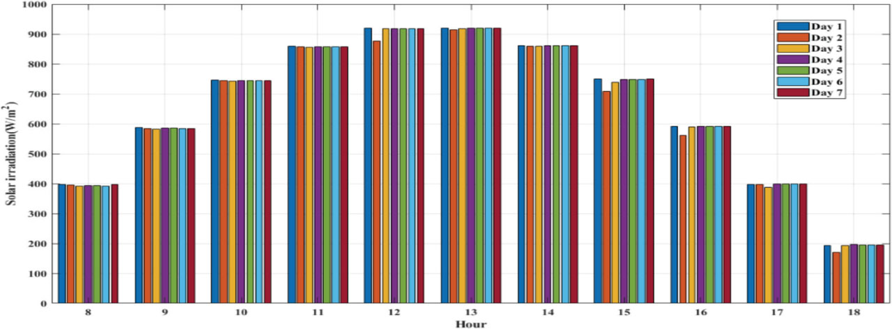
Figure 17.
Real hourly solar irradiance profiles of 7 days record.
The average measurements profile comprises 11 solar irradiance points presented in Figure 18a, revealing a marked solar peak between 12:00 pm and 1:00 pm, consistent with the region’s summer conditions. The average value of this vector is 676 W/m2, confirming the particularly high intensity of solar radiation during this period. Simultaneously, wind speed was measured at 10 consecutive hours, as shown in Figure 18b, with a calculated average value of 13 km/h, corresponding to a moderate wind regime typical of Gafsa’s semi-arid climate.
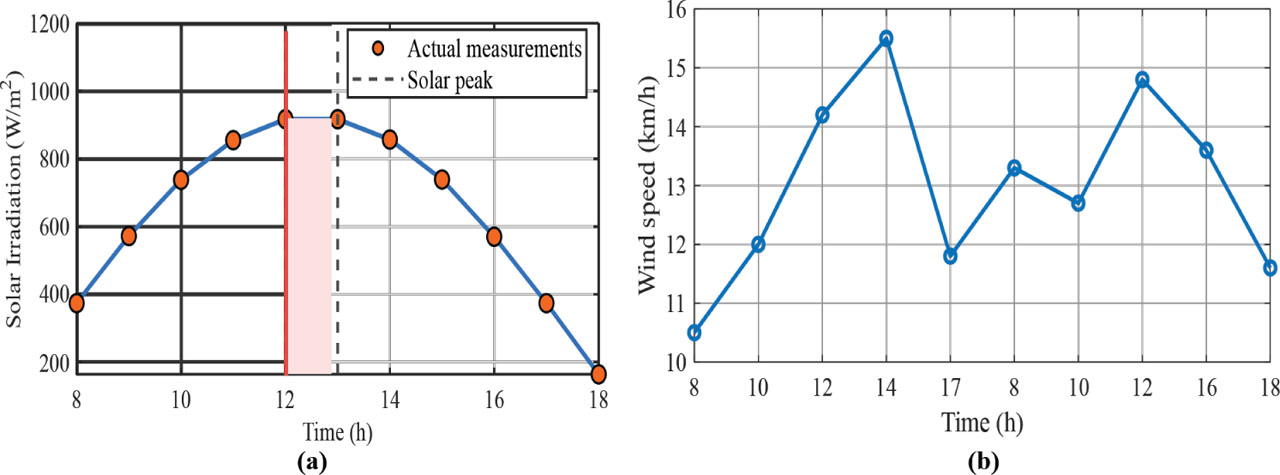
Figure 18.
Profile for solar irradiance and wind. (a) Solar irradiance. (b) Wind profile.
For the purposes of modelling in MATLAB/Simulink, the actual 10-hour time interval was resampled to a total duration of 2 seconds, resulting in a time step equivalent to 0.2 seconds per hour. This scaling choice significantly reduces computation time while preserving the dynamic nature of the measured profiles. In the initial configuration of the simulation, the SOC of the battery was set at 60%, while the domestic consumption profile was modelled as a variable load between 3 kW and 13 kW, with a notable peak between 12 pm and 3 pm, a period corresponding to the maximum of residential energy demand in the Gafsa region.
Figure 19 shows the average power produced by the two renewable energy sources in the microgrid. The wind source delivers an average power of approximately 30.6 kW, while the photovoltaic source delivers an average power of 4 kW.
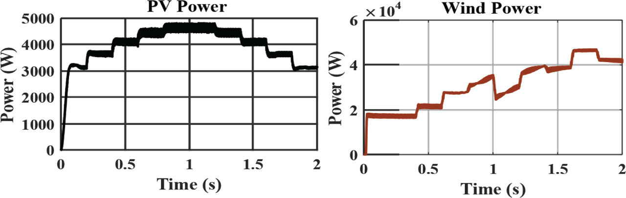
Figure 19.
Realistic renewable power generation.
A detailed analysis of the battery state, including the evolution of SOC, current, and voltage, is presented in Figure 20 for the FL control and in Figure 21 for the ANN control.
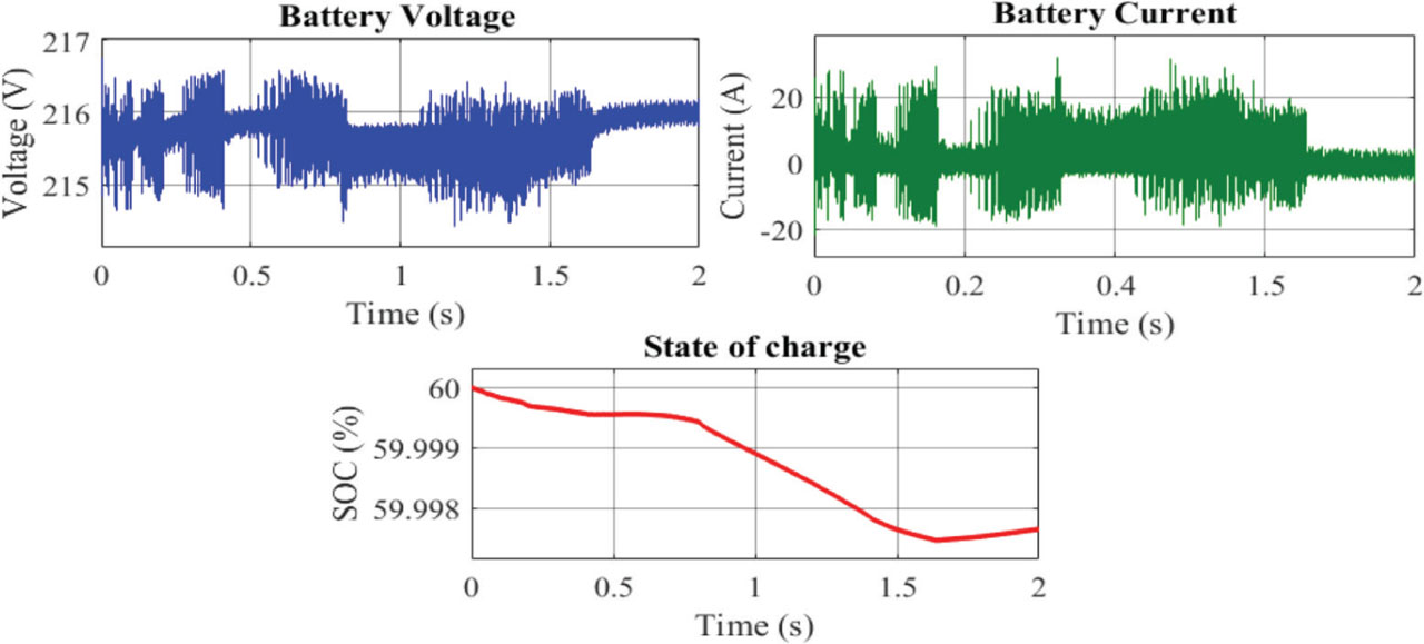
Figure 20.
FL battery state. SOC, state of charge.
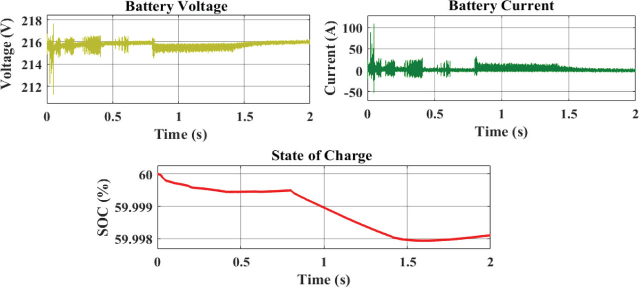
Figure 21.
ANN battery state. ANN, artificial neural network; SOC, state of charge.
The SOC remains within a narrow range, indicating stable short-term operation of the battery. However, noticeable oscillations in the battery current can be observed, reflecting the reactive nature of the FL controller when responding to instantaneous power variations. These current fluctuations are directly reflected in the voltage profile, which shows corresponding dynamic variations. This behaviour highlights the ability of the FL controller to provide rapid power support, though with increased short-term battery solicitation.
Compared to FL control, the SOC evolution appears smoother, with reduced oscillations over the simulation horizon. The battery current exhibits lower peak values and fewer fluctuations, indicating a smoother power regulation mechanism. Consequently, the voltage profile remains more stable. These results demonstrate the conservative nature of the ANN strategy, which effectively reduces short-term current fluctuations while maintaining stable battery operation under the considered simulation conditions.
Figure 22 compares the SOC trajectories under FL and ANN control for the same initial SOC condition. Both controllers maintain the SOC within acceptable operating limits, confirming the stability of the proposed battery management strategies.
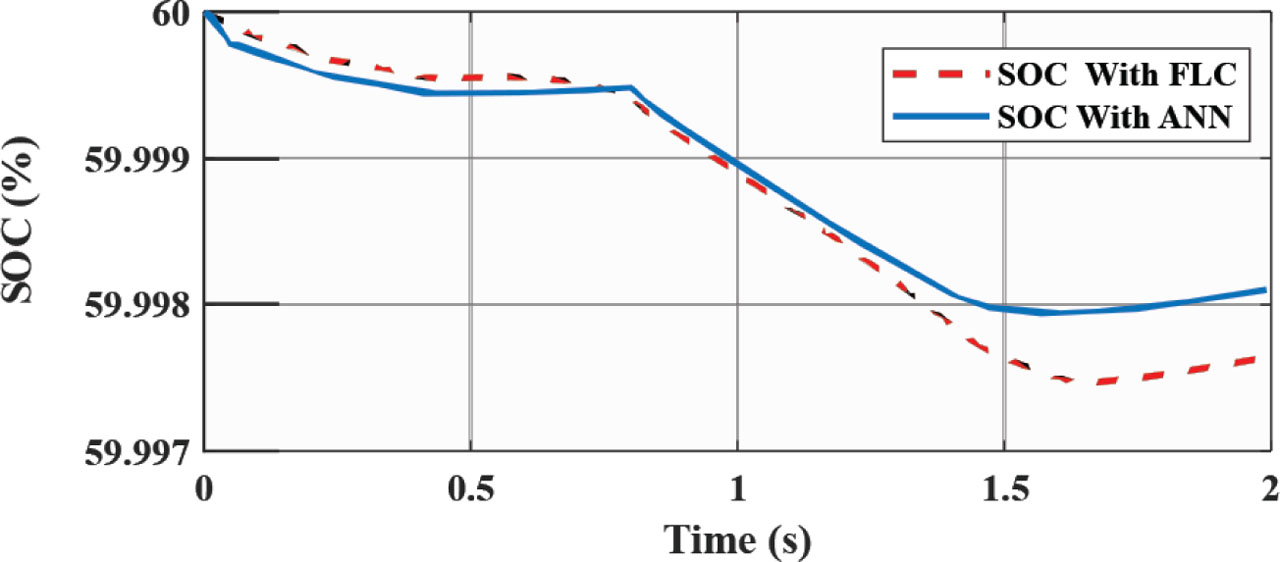
Figure 22.
SOC comparison: FL vs ANN. ANN, artificial neural network; FL, fuzzy logic; SOC, state of charge.
The SOC RMS demonstrates that ANN control reduces SOC fluctuations by 22.9% relative to FL control, confirming improved dynamic smoothness and lower battery stress.
Figure 23 compares the battery current profiles obtained under FL and ANN control. The peak current under FL control is noticeably higher than that obtained with ANN, confirming the more aggressive behaviour of the FL strategy.
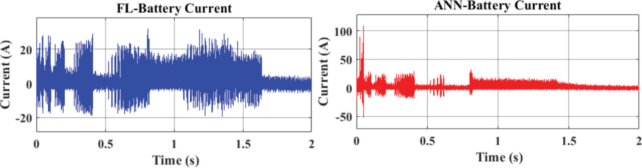
Figure 23.
Current comparison: FL vs ANN.ANN, artificial neural network; FL, fuzzy logic.
The FL controller exhibits higher current peaks and more pronounced oscillations, indicating a more aggressive dynamic response. However, the ANN-based controller produces a smoother current waveform with reduced fluctuations, reflecting lower short-term battery current behaviour.
4.4. Comparative study
To ensure a rigorous and unbiased assessment of the two proposed control approaches, numerical simulations were carried out under demanding battery operating conditions, specifically at low and high SOC levels. Two representative operating points were selected: case 1, SOC (%) = 20%, corresponding to a deeply discharged state in which the battery exhibits increased sensitivity to current variations, power constraints, and combined electrothermal stresses. Case 2 SOC (%) = 80%, representing a highly charged condition where the battery approaches saturation. This operating region is particularly critical due to the rise in internal resistance and the amplification of voltage fluctuations.
The performance comparison was conducted over a short simulation horizon of 2 seconds, emphasising the transient and dynamic response of the control strategies rather than long-term efficiency metrics. The obtained results are summarised in Table 8.
Table 8.
Comparative performance.
| Case | Metric | FLC | ANN | ANN improvement vs. FLC |
|---|---|---|---|---|
| Case 1 | Discharge energy (Wh) | 0.3646 | 0.3001 | 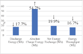 |
| Absolute charge energy (Wh) | 0.1270 | 0.1965 | ||
| Net energy exchange (Wh) | 0.2376 | 0.1905 | ||
| Energy throughput (Wh) | 0.4916 | 0.4098 | ||
| Case 2 | Discharge energy (Wh) | 0.3846 | 0.3159 | 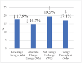 |
| Absolute charge energy (Wh) | 0.1285 | 0.1096 | ||
| Net energy exchange (Wh) | 0.2561 | 0.2062 | ||
| Energy throughput (Wh) | 0.5130 | 0.4255 | ||
| Overall | SOC RMS fluctuations | - | - | 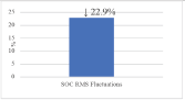 |
Based on the simulation outcomes for initial SOC conditions, the net energy assessment indicates that the FL controller imposes a greater demand on the battery compared to the ANN-based strategy. Although both control methods exhibit a predominantly discharge-orientated behaviour, the ANN controller consistently limits the amount of net energy exchanged with the battery. This observation reflects the more conservative operating nature of the ANN approach, whereas the FL controller tends to deliver more aggressive power support. Overall, the ANN-based strategy achieves an approximate 18% reduction in total exchanged energy relative to the FL controller, indicating smoother power modulation and reduced short-term battery loading. This distinction is especially pronounced at low SOC (20%), where the ANN controller more effectively constrains battery usage, suggesting enhanced protection under critical operating conditions.
Compared with the FL approach, the ANN-based battery management scheme demonstrates superior short-term performance in terms of battery utilisation. While the FL controller responds more aggressively by supplying higher instantaneous power levels, it also exhibits more frequent charge/discharge transitions and large current fluctuations. Conversely, the ANN controller ensures smoother power transitions and lower energy throughput, thereby mitigating battery stress and supporting improved battery preservation. Consequently, the ANN-based strategy offers a more favourable balance between dynamic responsiveness and stable battery operation, making it well suited for short-term battery management during transient operating scenarios.
4.5. Economic analysis
In order to quantify the specific economic benefits of FL and ANN control, a simplified cost study was conducted. The analysis demonstrates that, despite a steady load demand, minimising operational costs relies on intelligent battery storage management, directly influencing the system’s energy balance.
For the operating costs evaluation, the energy throughput indicator is used as the main parameter. Precisely, a high throughput implies greater stress on the storage system, leading to increased energy losses and a potential increase in costs related to battery wear.
The energy cost is calculated by using the following equation:
Where Ce represents the electricity price fixed at 0.414 Dt for a monthly residential consumption exceeding 500 kWh.
Two scenarios were studied (SOC (%) = 20% and SOC (%) = 80%). The results presented in Table 9 indicate that the ANN method exhibits lower energy throughput, directly resulting in reduced energy costs. The reduction achieved was 16.6% for the first case and 17.0% for the second.
Table 9.
Energy cost results.
| AI algorithm control | Energy throughput (KWh) | Cost (Dt) | Reduction (%) | |
|---|---|---|---|---|
| SOC = 20% | FLC | 0.0004916 | 0.0002035 | 16.60 |
| ANN | 0.0004098 | 0.0001697 | ||
| SOC = 80% | FLC | 0.0005130 | 0.0002124 | 16.99 |
| ANN | 0.0004255 | 0.0001762 |
This improvement confirms that the ANN algorithm better optimises energy flows while limiting unnecessary battery usage, which can contribute to improving overall profitability and reducing short-term battery stress.
5. Conclusion
This article presents the modelling and performance evaluation of a smart microgrid configured for the specific climatic and operational conditions of the Gafsa region in Tunisia. The integration of real-world data ensures a faithful characterisation of the system dynamics. A rigorous comparative analysis of BMS was conducted by comparing an FL controller with an ANN approach. The obtained results show that under the adopted short-term time-scaled simulation conditions, the FL controller provides higher instantaneous power support but exhibits more frequent charge/discharge transitions and larger current fluctuations. Conversely, the ANN approach ensures smoother power regulation and optimised flow management, resulting in a 17% reduction in energy costs compared to the FL solution. Quantitative evaluation demonstrates that the ANN-based controller achieves a 22.9% reduction in SOC RMS fluctuations while simultaneously minimising energy throughput and net energy exchange across both investigated scenarios (SOC = 20% and SOC = 80%). These findings demonstrate the superior short-term performance of the ANN-based BMS, providing a more stable battery current profile and smoother battery operation under the considered operating conditions. Although marginal increases in peak current may occur during brief transient phases, the ANN control framework consistently provides stable system operation throughout the simulated scenarios.
From a regional socio-economic perspective, the implementation of AI-driven microgrids offers a viable solution to the energy resilience challenges of Gafsa, particularly for mitigating load shedding during peak summer demand. Subsequent investigations aim to extend the BMS functionality by incorporating long-term degradation models and will be subjected to rigorous experimental verification using real-time and hardware-in-the-loop (HIL) platforms.