

Figure 1.
An example of steel sheet cutting on MPL. Source: Siemens AG (2025). MPL, material processing lines.
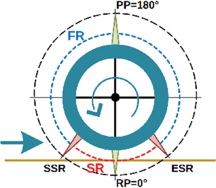
Figure 2.
Important areas of rotary shears trajectory. Source: Siemens AG (2025). ESR, end of the synchronous range; FR, formatting range; PP, parking position; RP, reference point; SR, synchronous range; SSR, start of the synchronous range.
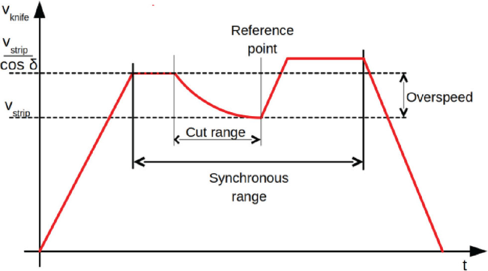
Figure 3.
Ideal shears trajectory during the cutting process. Source: Ďurovský et al. (2023).
Table 1.
Shears’ position and torque during cut.
| Parameters | Shears’ angle (°) | Shears’ arm (mm) | Torque on motor side | |
|---|---|---|---|---|
| (Nm) | (% of TR) | |||
| Beginning of cut | 339 | 34.045 | 1,872.2 | 76.14 |
| End of cut | 345 | 24.588 | 1,352.1 | 55 |
Table 2.
The shears’ angular velocity drop during the cut considering freewheeling shears (i.e. without controllers).
| Steady state (rad/s) | After cut (rad/s) | Difference (rad/s) | Difference (%) | |
|---|---|---|---|---|
| 20 | 14.74 | 7.63 | 7.11 | 48.34 |
| 50 | 36.847 | 34.021 | 2.862 | 7.77 |
| 80 | 58.938 | 57.180 | 1.758 | 2.98 |
Table 3.
Rotary shears motor parameters.
| Parameters | Symbol | Unit | Value |
|---|---|---|---|
| Rated power | PR | kW | 190 |
| Rated voltage | VR | V | 400 |
| Rated speed | nR | rpm | 800 |
| Motor inertia | Jmot | kg/m2 | 4.2 |
| Rated current | IR | A | 335 |
| Rated frequency | fR | Hz | 27.2 |
| Rated torque | TR | Nm | 2,328 |
| Maximum torque | Tmax | Nm | 4,250 |
| Rated power factor | cos(ϕ) | - | 0.942 |
| Rated efficiency | η | % | 89 |
| Torque control loop time constant | τT | ms | 2 |
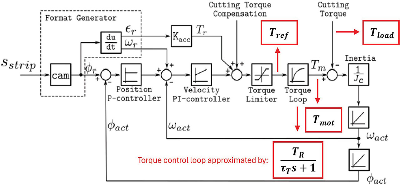
Figure 4.
The rotary shears control structure. Source: Ďurovský et al. (2023).

Figure 5.
Compensation torque and actual cutting torque during the shearing process.

Figure 6.
Structure fuzzy controller.

Figure 7.
Membership functions of the inputs and output. NM, negative medium; NS, negative small; PM, positive medium; PS, positive small.
Table 4.
Fuzzy control rules.
| e(k)/Δe(k) | NM | NS | Z | PS | PM |
|---|---|---|---|---|---|
| NM | NM | NM | NM | NS | Z |
| NS | NM | NM | NS | Z | PS |
| Z | NM | NS | Z | PS | PM |
| PS | NS | Z | PS | PM | PM |
| PM | Z | PS | PM | PM | PM |
Table 5.
Parameters of NN predictive model.
| Parameters | Value/description |
|---|---|
| Network type | Feedforward NN (MLP) |
| Output | Prediction of motor torque |
| Input vector | [Tref (k), Tref (k − 1), Tmot (k), Tmot(k − 1), Tload (k), Tload(k − 1)] |
| Hidden layers | 2 |
| Number of neurons | 10–10 |
| Activation functions | Tansig (hidden layers), linear (output layer) |
| Training algorithms | Levenberg–Marquardt |
| Input and output normalisation | Range [−1, 1] |
| Sampling period | Ts = 100 μs |
Table 6.
Performance metrics of the NN torque predictor.
| Abbreviation | Full name | Value | Unit |
|---|---|---|---|
| MAE | Mean absolute error | 1.7645 | Nm |
| RMSE | Root mean square error | 2.3071 | Nm |
| RMSE | Percentage RMSE | 0.0991 | % |
| MaxE | Maximum absolute error | 5.7528 | Nm |
| R2 | Coefficient of determination | 0.9999 | - |

Figure 8.
Detailed view of torque prediction error between view of torque prediction error between NN output and measured torque. NN, neural network.
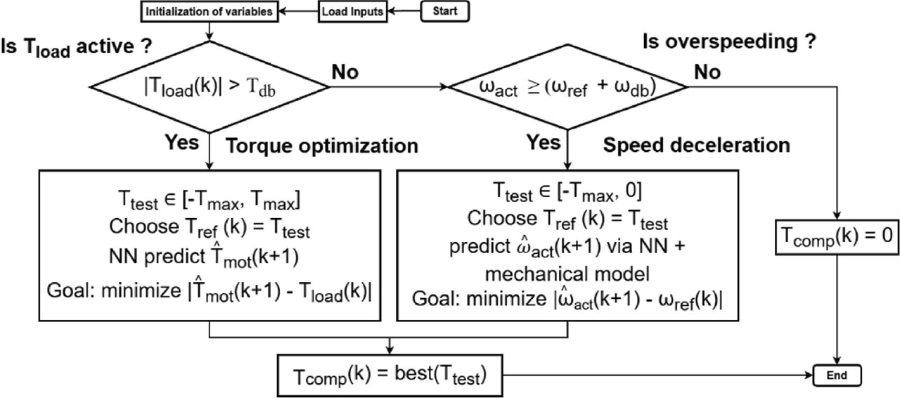
Figure 9.
Flowchart of the NN-based torque compensation algorithm. NN, neural network.

Figure 10.
Input signals used for NN training in the time domain. NN, neural network.

Figure 11.
Comparison of the 1D lookup-table-based compensation torque and the load torque. LUT, lookup table; NN, neural network.

Figure 12.
Simulation results of cutting 3 mm thick and 1,600 mm wide strip at 40 m/min. (a) P-type controller without compensation, (b) PI-type controller without compensation, (c) P-type controller with compensation, (d) P-type controller with anticipative compensation, (e) P-type controller with Fuzzy feedforward, (f) P-type controller NN-based LUT compensation. LUT, lookup table; NN, neural network.
Table 7.
Summary of dynamic performance metrics for all tested control structures and compensation strategies at different strip speeds.
| Strip speed [m/min] | Control structure | Compensation | Speed drop [%] | Absolutely speed drop [m/min] | Speed overshoot [%] | Settling time [ms] |
|---|---|---|---|---|---|---|
| 20 | P | No | 10.71 | 2.144 | 0.115 | 54.2 |
| PI | No | 9.12 | 1.824 | 1.534 | 82.3 | |
| P | Yes | 4.74 | 0.948 | 4.38 | 50.1 | |
| P | Anticipative | 5.71 | 1.143 | 4.21 | 50.7 | |
| P + fuzzy | No | 1.66 | 0.332 | 0 | 34.7 | |
| P | NN compensation | 1.07 | 0.214 | 0.06 | 35.7 | |
| 40 | P | No | 5.03 | 2.014 | 0.32 | 34.5 |
| PI | No | 4.35 | 1.740 | 4.48 | 53.1 | |
| P | Yes | 1.16 | 0.464 | 1.62 | 25.5 | |
| P | Anticipative | 0.78 | 0.311 | 1.58 | 16.6 | |
| P + fuzzy | No | 0.86 | 0.344 | 0 | 16.2 | |
| P | NN compensation | 0.55 | 0.222 | 0.02 | 19.4 | |
| 80 | P | No | 2.28 | 1.825 | 0.13 | 23.5 |
| PI | No | 2.03 | 1.621 | 1.47 | 44.2 | |
| P | Yes | 0.56 | 0.448 | 0.52 | 19.8 | |
| P | Anticipative | 0.47 | 0.377 | 0.45 | 19.5 | |
| P + fuzzy | No | 0.43 | 0.344 | 0 | 8.3 | |
| P | NN compensation | 0.28 | 0.226 | 0.01 | 10 |