
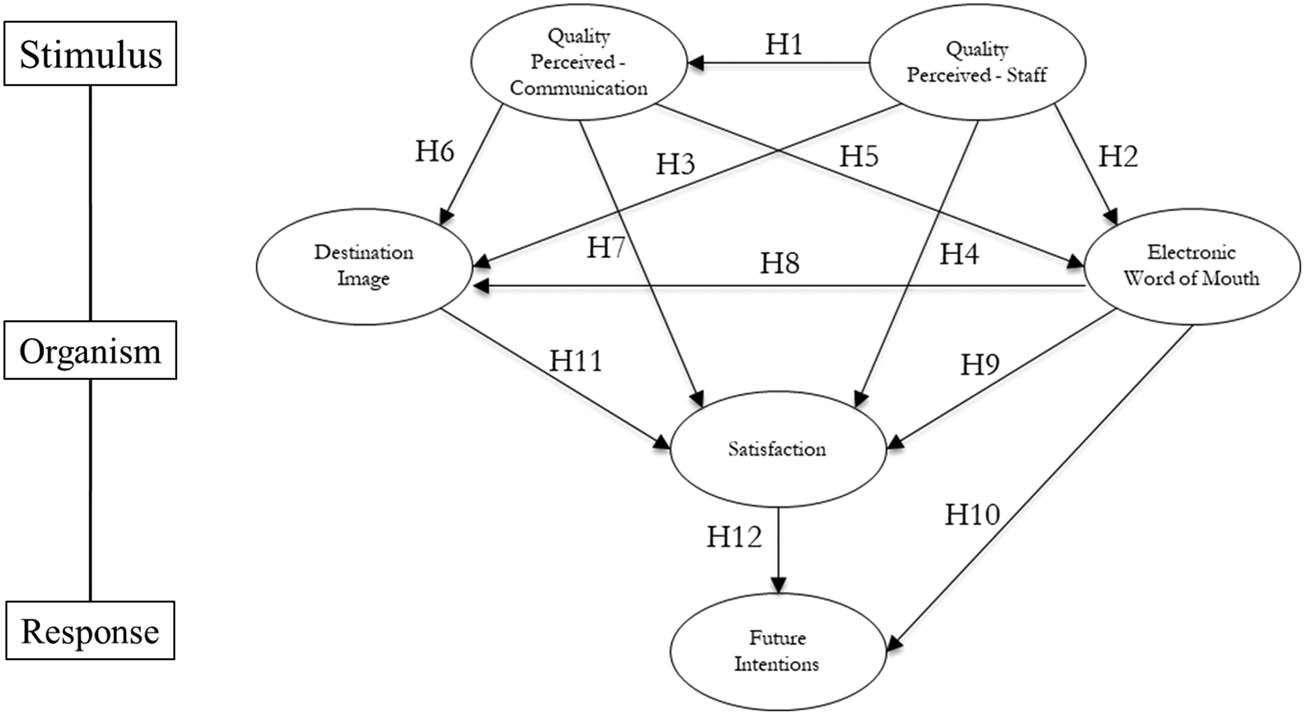
Figure 1
Research model.
Source: Authors’ contribution.
Table 1
Sample demographic profile.
| Characteristics | Frequency | |
|---|---|---|
| N (152) | % | |
| Gender | ||
| Female | 86 | 56.6 |
| Male | 66 | 43.4 |
| Age (years) | ||
| 18 to 30 | 42 | 27.6 |
| 31 to 45 | 59 | 38.8 |
| 46 to 60 | 38 | 25.0 |
| More than 61 | 13 | 8.6 |
| Marital status | ||
| Single | 53 | 34.9 |
| Married/Cohabited | 90 | 59.2 |
| Divorced/Separated | 8 | 5.3 |
| Widowed | 1 | 0.7 |
| Education level | ||
| Elementary studies | 14 | 9.2 |
| Junior High School | 18 | 11.8 |
| Senior High School | 24 | 15.8 |
| Professional education | 22 | 14.5 |
| Graduated | 58 | 38.2 |
| Post graduated | 16 | 10.5 |
| Occupation | ||
| Self-employed | 14 | 9.2 |
| Employed | 80 | 52.6 |
| Student | 40 | 26.3 |
| Unemployed | 8 | 5.3 |
| Retired/Pensioner | 7 | 4.6 |
| Housekeeper | 3 | 2.0 |
| Practice physical activity | ||
| Yes | 95 | 62.5 |
| No | 57 | 37.5 |
Source: Authors’ contribution.
Table 2
Measurement items, construct reliability and convergent validity.
| Abbreviations | Dimensions and items | Mean | SD | λ | |
|---|---|---|---|---|---|
| Quality Perceived – Communication (α = 0.74; CR = 0.76; AVE = 0.51) | |||||
| COM1 | The organization of the event provided me with a reliable, consistent, and dependable service | 6.21 | 1.07 | 0.611 | |
| COM2 | I had updated information about the event/participants/teams | 6.33 | 1.02 | 0.746 | |
| COM3 | The information about this event was easy to get | 6.17 | 1.04 | 0.775 | |
| Quality Perceived – Staff (α = 0.74; CR = 0.76; AVE = 0.51). | |||||
| STF4 | The event staff and the volunteers were competent | 5.99 | 1.21 | 0.705 | |
| STF5 | Staff behaviour was pleasant | 5.76 | 1.42 | 0.746 | |
| STF6 | The staff linked to the event made an effort to understand my needs and helped me with the questions I asked | 6.06 | 1.05 | 0.686 | |
| Electronic Word of Mouth (α = 0.79; CR = 0.83; AVE = 0.62) | |||||
| eWOM7 | Advertising of this event online was the key to choose this destination | 5.36 | 1.79 | 0.887 | |
| eWOM8 | I consulted and valued the comments and opinions I have read online when it came to choosing this destination | 5.23 | 1.79 | 0.838 | |
| eWOM10 | I search or I will search for publications by other attendees of this event on social networks | 4.95 | 1.96 | 0.609 | |
| Destination Image (α = 0.83; CR = 0.84; AVE = 0.64) | |||||
| DIM11 | There are good opportunities to enjoy free time and entertainment in the destination | 5.89 | 1.32 | 0.759 | |
| DIM12 | The destination offers interesting places to visit | 5.89 | 1.29 | 0.870 | |
| DIM13 | As a tourist destination, the place offers good value for money | 5.91 | 1.18 | 0.771 | |
| Satisfaction (α = 0.81; CR = 0.80; AVE = 0.57) | |||||
| SAT14 | I am having a good time attending this event | 6.14 | 1.07 | 0.823 | |
| SAT15 | I really enjoy attending sports events | 6.21 | 1.09 | 0.757 | |
| SAT16 | I think having free time and fun are important when it comes to choosing | 6.24 | 1.05 | 0.683 | |
| Future Intentions (α = 0.71; CR = 0.72; AVE = 0.56) | |||||
| FI17 | I am going to recommend this destination to my friends and relatives | 6.14 | 1.10 | 0.796 | |
| FI18 | If I had the opportunity to attend a similar sports event, I would repeat the experience | 6.32 | 1.12 | 0.696 | |
Note: all items are measured with a 7-point Likert scale anchoring strongly disagree (1) and strongly agree (7). SD = Standard Deviation, λ = item loadings, α = Cronbach’s alpha, CR = Composite Reliability, AVE = average variance extracted.
Source: Authors’ contribution.
Table 3
Discriminant validity analysis (Fornell–Larcker criterion).
| (1) | (2) | (3) | (4) | (5) | (6) | |
|---|---|---|---|---|---|---|
| Quality perceived – Staff | (0.51) | |||||
| Quality perceived – Communication | 0.42 | (0.51) | ||||
| Electronic Word of Mouth | 0.23 | 0.29 | (0.62) | |||
| Destination image | 0.39 | 0.36 | 0.28 | (0.64) | ||
| Satisfaction | 0.48 | 0.49 | 0.30 | 0.53 | (0.57) | |
| Future intentions | 0.45 | 0.49 | 0.35 | 0.52 | 0.46 | (0.56) |
Note: Values on the diagonal are AVE values, while the off-diagonal values are squared correlations between the constructs.
Source: Authors’ contribution.
Table 4
Path estimates.
| Path | Estimate | t Statistic | p-Value | Hypotheses |
|---|---|---|---|---|
| Staff → Communication | 0.748 | 5.325 | <0.001 | H1: supported |
| Staff → Electronic Word of Mouth | 0.181 | 1.037 | 0.300 | H2: not supported |
| Staff → Destination image | 0.341 | 2.252 | 0.024 | H3: supported |
| Staff → Satisfaction | 0.173 | 1.534 | 0.125 | H4: not supported |
| Communication → Electronic Word of Mouth | 0.404 | 2.292 | 0.022 | H5: supported |
| Communication → Destination image | 0.183 | 1.099 | 0.272 | H6: not supported |
| Communication → Satisfaction | 0.125 | 1.149 | 0.250 | H7: not supported |
| Electronic Word of Mouth → Destination image | 0.253 | 2.456 | 0.014 | H8: supported |
| Electronic Word of Mouth → Satisfaction | 0.077 | 0.931 | 0.352 | H9: not supported |
| Electronic Word of Mouth → Future intentions | 0.030 | 0.741 | 0.733 | H10: not supported |
| Destination image → Satisfaction | 0.603 | 6.663 | <0.001 | H11: supported |
| Satisfaction → Future intentions | 0.913 | 8.759 | <0.001 | H12: supported |
Source: Authors’ contribution.
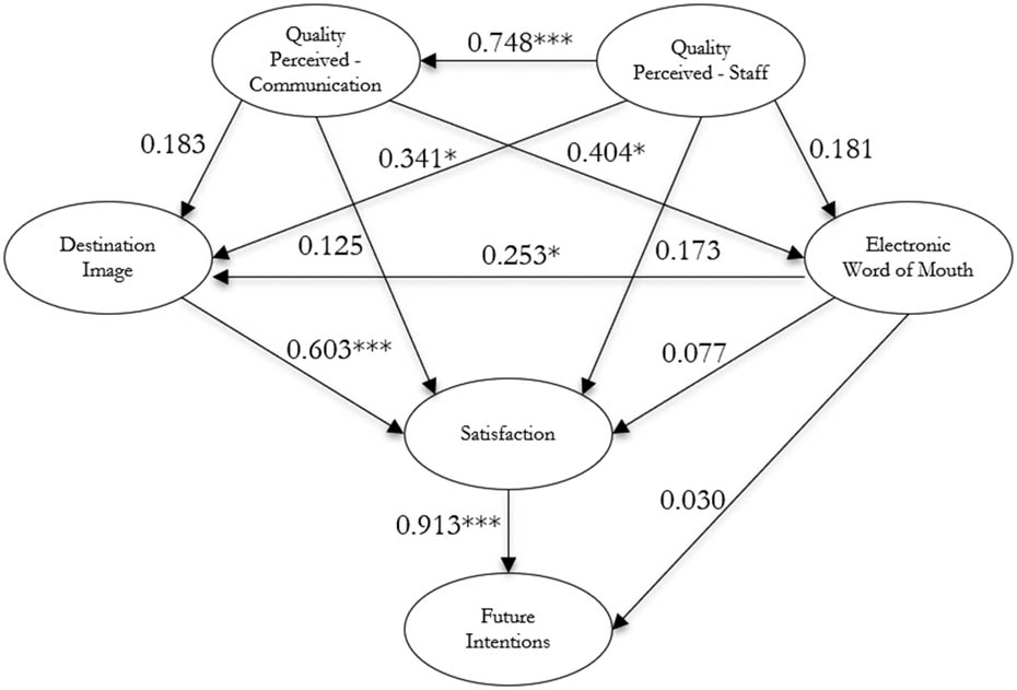
Figure 2
Model SEM coefficients and relations between variables.
Source: Authors’ contribution.