
One of the key decisions of any project is the choice of delivery method (Pakkala 2002; AIA California Council 2007). The project delivery method (PDM) should be coordinated with the requirements of building information modelling (BIM) to provide a suitable basis for reducing time and cost and increasing the quality of implementation, which is one of the main goals of information modelling (Ghassemi and Becerik-Gerber 2011). If the correct method of project delivery is not used, the goals of information modelling will not be achieved, and spending more money to benefit from this new approach of the construction industry will not help to achieve the goals of the project. For this purpose, coordinating the PDM with information modelling requirements is an inevitable necessity.
In the BIM guidelines, which are widely used, BIM technology and related processes for generating, communicating, and analysing building models are defined (Sacks et al. 2018). PDM is an agreement between the parties to obtain and provide services for a specific project (Miller et al. 2000). Researchers have compared different PDMs in terms of their impact on project performance. Most of them focus on design-build (DB), design-bid-build (DBB) (Hale et al. 2009), and construction management at risk (CMR) (Guo et al. 2014). It has been found that DB contracts have a positive and significant impact on cost and time savings compared to DBB (Hale et al. 2009). On the contrary, it has been found that CMR is more effective in saving time compared to DB (Molenaar et al. 2009). CMR and DB also reduce communication problems and disputes compared to the DBB method for infrastructure projects (Shrestha et al. 2016). Despite the advantages offered by a particular PDM, its choice is mainly related to the decision of the owner or client and the budget, duration, and type of project (Konchar and Sanvido 1998). DBB, DB, and CMR are also recognised as the dominant PDMs in the construction industry (Molenaar et al. 2009). It has been reported that customers’ understanding, knowledge, and skills are influential in choosing PDM (Mahdi and Alreshaid 2005).
The main determinants of these procurement models are as follows:
DBB: The project is designed entirely before construction begins, and construction contractors bid on the project based on the completed design.
DB: A single entity is responsible for design and construction, which can streamline communication and reduce project timelines.
CMR: A construction manager commits to completing the project within a guaranteed maximum price and takes on the risks associated with delivering the project on time and within budget.
Therefore, it can be stated that the choice of PDM or the priority proposed under a particular PDM is largely dependent on the characteristics of the organisation. These characteristics include organisational structure, financial stability, managerial expertise, technical capability, and previous experience with similar projects. For example, a financially stable organisation with experienced management and technical staff might prefer the DB model to leverage its in-house capabilities and reduce project duration.
Organisational characteristics have also been associated with awareness of integrated project delivery (Kent and Becerik-Gerber 2010). Despite the mentioned arguments, the effects of organisational characteristics on the choice of PDM have not been carefully investigated. In this work, the data of construction industry organisations in Iran are analysed regarding their selection of different PDMs.
Omar and Fayek (2016) modelled and evaluated construction projects, their merits, and their relationship with project performance. In this research, by examining 41 articles, 248 project merit criteria were extracted. Also, seven categories of performance factors with 46 criteria were extracted. The variables were identified and prioritised using the fuzzy method. The results of the factor analysis showed that the merits of the project affect its performance.
Kwofie et al. (2016) investigated the critical success factors of public-private partnership (PPP) projects in the delivery of housing in Ghana. In this research, he modelled the factors affecting the success of PPP in the delivery of housing in Ghana, and the results of the research showed that the beneficiaries in public and private projects have a major role in the implementation and delivery of the project.
Analysis of variance (ANOVA) and t-test were used to compare PDMs based on project performance and stakeholder ratings (Hale et al. 2009; Qiang et al. 2015). Mahdi and Alreshaid (2005) have used a multivariate regression model to predict the performance of projects with different PDMs.
Analytic hierarchy process (AHP), particle swarm optimisation, and multi-criteria utility theory have been used to develop decision support systems for customers to choose the right PDM for their project (Al Khalil 2002; Zeng et al. 2014). However, this study is focussed on creating a predictive model for the preference of organisations to deliver or implement projects under different PDMs. Therefore, the artificial neural network (ANN) is more useful in this field.
Many researchers have investigated the necessity of paying attention to BIM and identifying its problems and obstacles. Glick and Guggemos (2009) have considered modelling and integrated delivery of the project as two complementary arms that together guarantee the success of the project. In the guidelines and upstream documents related to BIM, the discussion of the compatibility of information modelling and the PDM has been considered (Sacks et al. 2018). Some researchers have paid attention to BIM platforms and have provided mechanisms to adapt platforms such as Vision as one of the most widely used information modelling platforms with the integrated project delivery system approach (Huahui et al. 2019).
Akinosho et al. (2020), in review research, discussed deep learning in the construction industry and the current situation and future innovations. Deep learning has been used for common construction challenges such as structural health monitoring, construction site safety, building occupancy modelling, and energy demand prediction. Matel et al. (2022) used an ANN to estimate engineering costs. The findings show that ANNs can obtain relatively accurate cost estimates, even with small datasets. In fact, the model presented in this article performed better than the proposed model in other similar works and showed a 14.5% improvement in model accuracy considering the mean absolute percentage error (MAPE).
Tijanić et al. (2020) investigated the cost estimation in road construction using an ANN. The contractor’s experience in previous road projects is an important element that can help prevent errors and increase the chances of success in similar projects in the future. Construction cost data collected from past projects can be used to estimate costs at different stages of the project life cycle through ANNs. In this article, ANNs (multilayer perceptron [MLP], generalised regression neural network [GRNN], and radial basis function neural network [RBFNN]) have been modelled to estimate road construction costs. Comparing the performance of neural networks has shown that GRNN with a MAPE of 13% and a determination coefficient of 0.9595 has achieved the best accuracy. Neural network has been proven to be a promising method to use in the initial design stage where there is usually a limited or incomplete dataset for cost analysis, and this method can produce much more accurate results and reduce the estimation error.
Golnaraghi et al. (2019) used ANN(s) in predicting labour productivity. In this study, expected productivity was modelled according to environmental and operational variables. To choose the best method to estimate the efficiency of different ANN techniques including GRNN, backpropagation neural network (BNN), RBFNN, and adaptive fuzzy neural inference system (ANFIS) to compare the relevant results were used. The results show that BNN performs better than other construction labour productivity modelling techniques. Juszczyk and Leśniak (2019) modelled the construction site cost index based on neural network groups. The results showed that the developed models based on the group average and cumulative generalisation meet the expectations of knowledge generalisation and accuracy of site overhead cost index prediction. The proposed models provide cost prediction within an accepted error range and prove to provide better predictions than individual neural networks. The developed tools can be used in the decision-making process regarding construction cost estimation.
Fischer et al. (2017) have also discussed the integrated project delivery system from various perspectives such as integration between all actors, value creation, and leadership of integrated teams and have provided operational guidelines for it. El-Sawalhi and Shehatto (2014) used a neural network model to estimate the cost of construction projects. The results showed that the neural network model succeeds in estimating the cost of construction projects without the need for more detailed maps. The average percent error of the tested dataset for the adapted model was largely acceptable (<6%). The sensitivity analysis showed that the typical floor area and the number of floors are the most important parameters in the building cost. The influence of individual input variables on the output variables was assessed through a sensitivity analysis. This analysis revealed that financial stability and managerial expertise had the most significant impact on predicting the correct PDM.
The aim and purpose of this work are to develop a predictive model using ANN to determine the most suitable PDM based on organisational characteristics. This research is focussed on the construction industry in Iran. The decision to use a neural network in this research is due to its ability to handle complex, non-linear relationships between variables, which are common in predicting project outcomes based on multifaceted organisational characteristics (Kulkarni et al. 2017). Neural networks can provide higher accuracy and better generalisation compared to traditional statistical methods (Jain and Pathak 2014).
In reviewing the literature, it was observed that while much research has been done on the comparison of different PDMs, there is a gap in understanding how organisational characteristics influence the choice of PDM. This study aims to fill this gap by analysing data from construction industry organisations in Iran and providing a model that predicts the optimal PDM based on these characteristics. The novelty of this work lies in its focus on organisational characteristics as predictors for PDM choice and the application of ANN for this purpose.
First, the theoretical foundations and related research were reviewed to identify effective organisational characteristics in predicting the correct method of project delivery. After that, the validation of the identified indexes was done through the Delphi technique. In the next step, quantitative data were collected via questionnaires and analysed using the ANN data mining algorithm. Finally, the accuracy of the neural network model was compared with other data mining models to highlight its effectiveness and demonstrate its superior performance in predicting the optimal PDM.
The flowchart of the study process of this research is illustrated in Figure 1. The study began with a literature review and exploratory studies to identify potential project delivery indexes and design the initial model. This was followed by the Delphi method to refine these indexes with an expert input. After finalising the indexes, a survey was conducted with a larger sample to collect quantitative data. The data were then analysed using the ANN model, and the model’s accuracy was compared with other data mining techniques. So, the final model is presented using surveys and ultimately applied to construction companies in the province, where the results are examined.
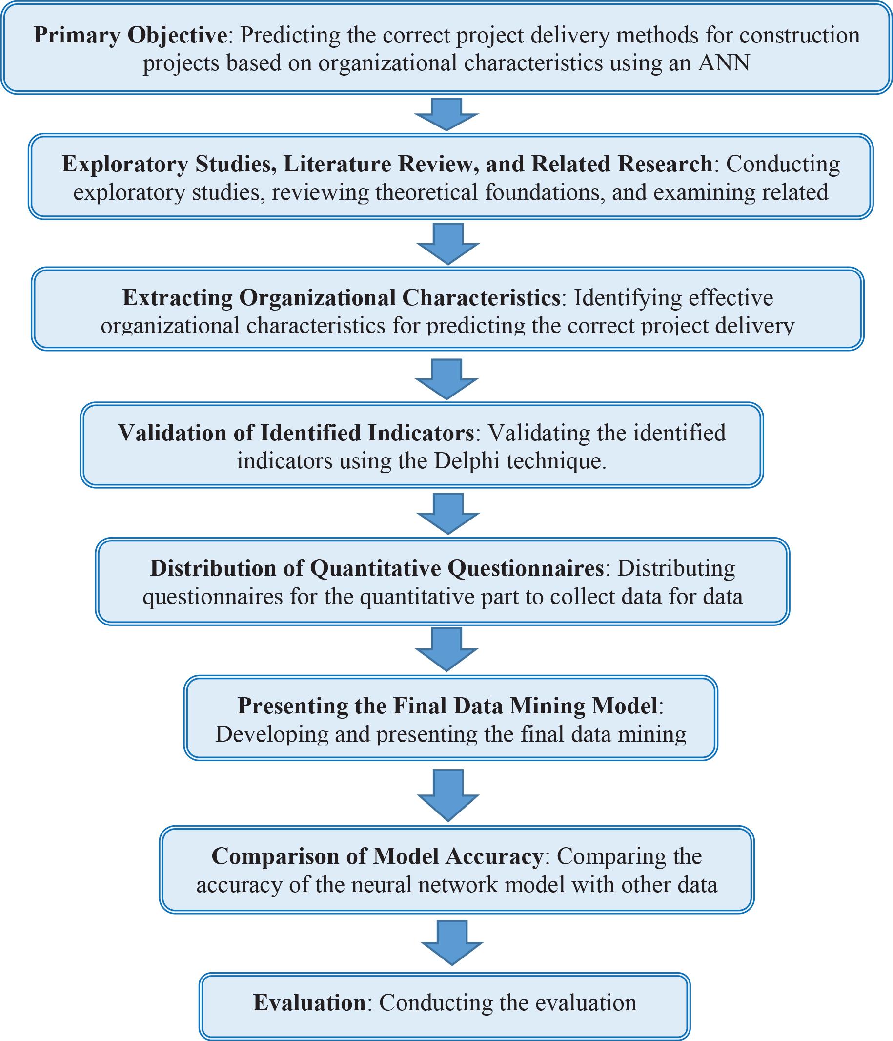
The general process of this research. ANN, artificial neural network.
The following key steps, which are explained in detail within its corresponding subchapter, outline our comprehensive approach.
A comprehensive literature review was conducted to identify the key organisational characteristics influencing PDMs. The variables were derived from existing research and validated through an expert input via the Delphi method. The library method and Delphi technique were used to extract and screen project delivery indexes by the company. Project delivery indexes refer to the specific criteria and characteristics used to evaluate and predict the appropriate method of project delivery. These indexes include various factors related to organisational structure, financial stability, managerial expertise, technical capability, and project experience. Each of these factors is assessed to determine their impact on the success and appropriateness of different PDMs. The statistical population in this research includes the following two groups:
The first group: Statistical population including construction experts related to the identification of effective organisational characteristics in predicting the correct method of project delivery (qualitative part).
The second group: The statistical community of construction experts in the study (quantitative part).
The Delphi method was employed to refine and validate the identified variables. This process involved multiple rounds of feedback from a panel of experts. This method included the calculation of the content validity ratio (CVR) to ensure the validity of the identified variables.
- –
First round: Initially, 20 experts from the construction industry with relevant knowledge and expertise were invited to participate in the Delphi method. In the first round, the list of levels, dimensions, and indexes of the model was provided to Delphi members for comments, suggestions, and modifications of the indexes. After the first round, 15 experts continued, and by the final round, 10 experts provided their feedback and consensus. The criterion for selecting experts in this research is that the first group of experts with good work records at high academic levels were used.
- –
Second round: After collecting the results of several deletion options, several combinations and modifications were made based on expert feedback. The revised structure was presented to the experts in the second round.
- –
Third round: In this round, the panel reached a suitable consensus on the final model. The final model was explained according to the obtained results and confirmation of the levels, dimensions, and indexes of the last stage. At the end of each stage, the researcher made the necessary corrections according to the opinions of Delphi experts. The results of each stage were summarised and reported to the experts in the subsequent stage, including the mean, mode, and median of the results (Linstone and Turoff 1975).
According to the results of the review of library studies, 35 variables were identified. After extracting the variables, the validity of the identified variables was checked and confirmed using the Delphi technique and experts’ opinions. The goal of this method is to reach the most reliable agreement of a group of experts on a specific topic, which is done by using a questionnaire and asking experts for their opinions many times according to their feedback.
The significance level in the Delphi method was set at 0.05, meaning that any index with a p-value >0.05 was excluded from the next round. The CVR was used to quantify the necessity of each item, calculated as:
In this research, after analysing the obtained data, relevant indexes, components, and dimensions were extracted. Then, by sending a questionnaire and obtaining answers, summarising, preparing the second questionnaire, sending it, and repeating this process, the work was carried out. This process continues until the result (pattern) of the work is reached. The implementation process of the Delphi method is shown in Figure 2.
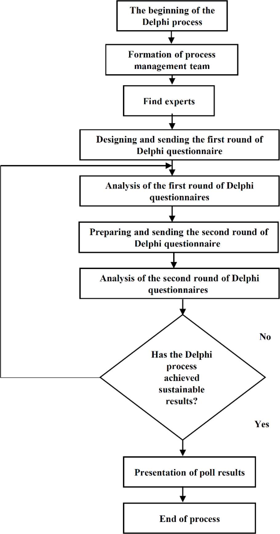
Delphi executive process.
The target population for the quantitative part of the study consisted of 360 construction experts from the Mazandaran province, Iran. Using Cochran’s formula, 354 participants were selected through the random sampling method. Cochran’s formula is used to determine the sample size for a survey. It is given by:
The questionnaires were developed based on the validated variables and indexes from the Delphi method. The data-gathering tool included structured questions designed to capture detailed information about organisational characteristics influencing PDMs.
The variables and indexes in the questionnaires were obtained based on an extensive literature review and expert opinions gathered through the Delphi method. This process involved identifying key organisational characteristics, which were validated and refined through multiple rounds of expert feedback. The questionnaires used for both groups of respondents consisted of structured questions. The questions were designed based on an extensive literature review, including sources such as Al-Shamsi (2013); Ahlemann et al. (2021); Kerzner (2022). The Delphi questionnaire included closed questions rated on a 5-point Likert scale and open-ended questions for additional comments. The survey questionnaire for the quantitative part included questions on organisational structure, financial stability, managerial expertise, and project experience.
Data were collected from the selected sample using the developed questionnaires. The respondents’ demographics included a mix of project managers, engineers, and senior management, with an average of 15 years of industry experience. The collected data (responses from 354 construction experts) provided a robust dataset for analysis. Statistical indicators such as mean, standard deviation, and frequency distributions were calculated to understand the central tendencies and variability within the data.
To determine the reliability of the questionnaires, first, 30 people were selected from the statistical population, and the questionnaire was given to them. Then, the Cronbach’s alpha method was used to determine the reliability (Collins 2007). For this purpose, to calculate the Cronbach’s alpha coefficient, first, the variance of the scores of each subset of the questions in the questionnaire (or sub-test) and the total variance should be calculated, and then, the value of the alpha coefficient should be calculated using the following equation (Nunnally 1994; Tavakol and Dennick 2011):
The inputs of this study were evaluated based on identified organisational characteristics, including financial, managerial, contextual, optimisation, and manpower variables. The outputs were the predicted PDMs. Data collection for these inputs and outputs was conducted using a Likert scale in the questionnaires, where respondents rated each characteristic on a scale from 1 (strongly disagree) to 5 (strongly agree). The data collection involved rating the inputs and outputs using specific units for evaluation. For the Delphi method and quantitative survey, a 5-point Likert scale was employed. Respondents were asked to rate various organisational characteristics and their influence on PDMs on a scale from 1 to 5, where:
1 = Strongly disagree
2 = Disagree
3 = Neutral
4 = Agree
5 = Strongly agree
The inputs (organisational characteristics) were rated by the respondents. The outputs were the effectiveness and appropriateness of different PDMs (e.g., DB, DBB, and CMR) as perceived by the respondents.
The collected data were normalised and used as input features for the ANN model. The normalisation process ensured that the data were on a similar scale, which is essential for the effective training of the ANN model.
In sum, the database creation process in this research involved the following steps:
Identification of variables:
- ο
Key organisational characteristics were identified through the Delphi method and literature review. These included managerial expertise, financial stability, technical capability, project experience, and contextual factors.
- ο
Data collection tool:
- ο
Structured questionnaires with a Likert scale were used to rate various organisational characteristics and their influence on PDMs.
- ο
Data normalisation and input preparation:
- ο
The responses were normalised to ensure that they were on a similar scale.
- ο
Database composition:
- ο
The final database included responses from some construction experts, providing a robust dataset for the analysis. The database was structured to include inputs (organisational characteristics [e.g., financial stability and managerial expertise]) and outputs (PDMs [e.g., DB, DBB, and CMR]).
- ο
Validation and reliability:
- ο
The reliability of the data collection tools was ensured using Cronbach’s alpha. This step ensured that the data collected were consistent and reliable for model development.
- ο
The ANN model was used to predict the optimal PDM based on the organisational characteristics. The ANN model was implemented using RapidMiner software, RapidMiner, Inc., Boston, MA, USA.
ANNs are a class of machine learning methods that have been developed in the fields of statistics and artificial intelligence and have regression and classification capabilities. The basis of this method is modelled on the complex neural networks in the human brain. In this study, the ANN model was designed to predict the optimal PDM based on the identified organisational characteristics.
Generally, the framework of neural networks consists of several layers called input layer, hidden layer(s), and output layer (Figure 3).
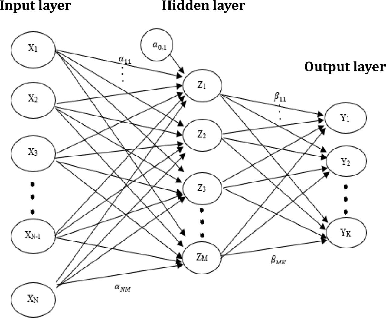
The structure of a neural network with one hidden layer.
Each layer contains components called neurons or nodes. The sets of {X1, X2, …, XN}, {Z1, Z2, …, ZM}, and {Y1, Y2, …, YK} are the set of nodes of the input layer, the set of nodes of the hidden layer, and the set of nodes of the output layer, respectively. Each of the existing connections between two nodes is carried out with a certain weight (coefficient). It is also possible in a neural network, in addition to the values of the nodes in the previous layers, which are assigned to a specific node in the next layers, to have a value entered as an oblique value to that particular node. In general, it can be said that α0m and β0k are the skewness values that, respectively, enter the nodes Zm and Yk. αim and βmk are, respectively, the weights of the connectors that connect the node Xi to Zm and the node Zm to Yk.
Depending on the type of explanatory and response variables, the number of nodes in the input and output layers is determined. In the input layer, one node is considered for each explanatory variable of quantitative type. In the output layer, for the regression mode, when we have K response variables, K nodes are considered, and for the classification mode with K categories, K nodes are considered in the output layer. The number of nodes in the hidden layers is chosen arbitrarily. The number of input variables, the type of combination function and activation function, and the way nodes are connected to determine the overall structure of a neural network. One of the most important structures used in this research is the MLP structure, which is a type of feedforward neural network (Gardner and Dorling 1998).
With a small number of nodes, the model may not have enough flexibility to represent non-linear properties in the data. On the contrary, the large number of nodes when the weight loss method is used to adjust the weights may cause the weights to approach zero. Therefore, choosing the number of nodes and hidden layers can have a great impact on the accuracy of a model. The best way to choose the best number of nodes and hidden layers is to use the trial and error method (Ripley 1996; Mitchell 1997). One of the main activation functions used in the neural network model is the sigmoid function. It is differentiable, which is necessary for backpropagation during the training of the network (Haykin 1998).
In our model, the dataset is divided into two parts: modeller (training) data and test data whose ratios are reported in the ‘Results and discussions’ section. Based on the data of the modeller, the modelling and parameter estimation of the model are done, and the accuracy of the model is checked using the test data.
The best-performing ANN model is determined to provide the highest accuracy among the various models tested, which are reported in the ‘Results and discussions’ section. The model architecture includes:
Input layer: Consists of five neurons, one for each predictor variable (organisational structure, financial stability, managerial expertise, technical capability, and project experience).
Hidden layer: Includes several neurons whose number is checked later in the ‘Results and Discussions’ section, and the appropriate value is selected (high accuracy).
Output layer: Consists of 12 neurons, corresponding to the number of PDMs.
The coefficients related to the connection of nodes in the hidden and output layers are reported in the ‘Results and discussions’ section.
A statistical summary of the collected data is presented in Table 1. This summary includes the mean, standard deviation, and minimum and maximum values for each variable.
Statistical summary of the collected data
| Variable | Mean | Standard deviation | Minimum | Maximum |
|---|---|---|---|---|
| Managerial expertise | 3.8 | 0.7 | 2 | 5 |
| Financial stability | 3.5 | 0.8 | 1 | 5 |
| Technical capability | 4.0 | 0.6 | 2 | 5 |
| Project experience | 3.7 | 0.7 | 2 | 5 |
| Contextual factors | 3.6 | 0.8 | 1 | 5 |
The collected data were normalised to ensure consistency and comparability across different scales. The normalisation process involved transforming data values to fall within a specific range. The data were normalised using min-max normalisation, which scales the data to a fixed range, typically 0 to 1, ensuring that all input features contribute proportionately to the model (Table 2).
Example of normalised data
| Respondent ID | Managerial expertise | Financial stability | Technical capability | Project experience | Contextual factors |
|---|---|---|---|---|---|
| 1 | 0.75 | 0.80 | 0.60 | 0.70 | 0.65 |
| 2 | 0.60 | 0.55 | 0.75 | 0.65 | 0.70 |
| … | … | … | … | … | … |
| 354 | 0.80 | 0.70 | 0.85 | 0.75 | 0.80 |
The reliability of the data collection tools was ensured using Cronbach’s alpha. The results are shown in Table 3.
Cronbach’s alpha coefficient for reliability analysis
| Construct | Cronbach’s alpha |
|---|---|
| Managerial expertise | 0.82 |
| Financial stability | 0.84 |
| Technical capability | 0.80 |
| Project experience | 0.83 |
| Contextual factors | 0.85 |
| Overall questionnaire | 0.85 |
According to the results table, the value of alpha for all constructs has a value >0.7, which indicates the validity of the questionnaire and the appropriate and equal intellectual perception of the respondents about the content of the variables related to each construct. The obtained Cronbach’s alpha coefficient for the entire questionnaire was 0.85, indicating high reliability.
In the first round, some variables did not meet the conditions to remain in the Delphi process and were removed from the analysis. The questionnaire was reloaded based on the remaining indexes and made available to the experts. In the second stage of Delphi, 10 questionnaires were distributed among the experts, and after 2 weeks of follow-up and at least three re-visits, 10 questionnaires were finally collected. The results of the second round show the significance and validity of all the remaining indexes. For remaining in the final model, both conditions of t-test and CVR value >62% are required, and as a result, the double rounds of Delphi can be ended.
The ANN model’s input variables, their types, descriptions, and indicators are detailed in Table 4. The dimensions of them are 1 (e.g., a Likert scale rating from 1 to 5).
Overview of input variables
| Variable | Type | Description | Indicators |
|---|---|---|---|
| Managerial expertise | Numerical | Measures the level of expertise and experience of the managerial team | Project management plan, supervision team management, coordination of planning, managerial support, adoption of new methods, and continuous monitoring and control |
| Financial stability | Numerical | Assesses the financial health and stability of the organisation | Timely payment, cost planning, planning and control system, project pricing, economic justification, and financial resource creation |
| Technical capability | Numerical | Evaluates the technical skills and capabilities of the organisation | Technical foundation, reporting systems, and optimisation programmes |
| Project experience | Numerical | Reflects the organisation’s experience with similar projects | Project management experience, training and development, and human resources satisfaction |
| Contextual factors | Numerical | Considers external factors that might impact project delivery | Infrastructure, legal obstacles, training, and culture development |
In addition to the primary variables listed above, this study also considered several specific indicators within these categories. These indicators were aggregated to form composite scores for each of the main variables. The indicators were quantified based on the responses to specific questionnaire items. The detailed indicators are:
Managerial expertise indicators
- ο
Existence of a comprehensive project management plan
- ο
Effective management by the supervision team
- ο
Coordination between planning and other units
- ο
Support from top and middle managers
- ο
Adoption of new planning methods by traditional managers
- ο
Continuous monitoring and control by the management team
- ο
Financial stability indicators
- ο
Timely payment at different project stages
- ο
Real cost planning aligned with project requirements
- ο
Implementation of project planning and control systems
- ο
Accurate project pricing
- ο
Examination of the economic justification of projects
- ο
Creation of new financial resources
- ο
Technical capability indicators
- ο
Use of appropriate technical foundation for energy optimisation
- ο
Implementation of new reporting systems
- ο
Development of comprehensive optimisation programmes
- ο
Project experience indicators
- ο
Experience and skill of the project management team
- ο
Training and development of project supervisors and managers
- ο
Satisfaction of the organisation’s human resources
- ο
Contextual factor indicators
- ο
Existence of the required infrastructure
- ο
Removal of legal obstacles
- ο
Training and culture development for project management
- ο
PDMs that play a role as response variables in the model include 12 methods as shown in Table 5. PDMs including various contracting strategies are derived from standard practices and frameworks used in the construction industry.
PDMs
| Escrow (one factor) |
| Percentage |
| Unit price |
| Price list (without aggregates or with aggregates) |
| MC |
| BOT |
| Purchase and installation |
| Design, purchase (procurement), and execution (Engineering, Procurement, and Construction – EPC) or design and construction |
| Project delivery systems |
| Multifactorial method (multiple prime) |
| Construction manager method |
| DB method |
BOT, build operate transfer; DB, design-build; MC, management contract; PDMs, project delivery methods.
So, the variables in the model are as below:
Predictor variables: The predictor variables in the model included financial stability, managerial expertise, technical capability, project experience, and contextual factors.
Target variables: The target variable was the PDM.
At first, the Read Excel operator is used to enter information into the Rapid Miner 5.1 software to perform data mining.
The dataset was divided into a training set (70% of the total data) and a test set (the remaining 30% of the data) using the validation operator in RapidMiner 5.1 software. In other words, from the total of 354 collected responses, 248 responses were used to train the model, and the remaining 106 responses were used to test and validate the model’s performance.
Accuracy criteria are used to select the best model. The prediction accuracy of the models is compared, and the best model is suggested in terms of accuracy. The accuracy criterion used to evaluate the ANN model’s performance was the percentage of correct predictions made by the model. To identify the best ANN model with the best number of hidden layers and the best number of neurons in the hidden layer, the neural network model with one to five hidden layers with different numbers of neurons in the hidden layer is fitted on the data. The results for the number of different layers and neurons are shown in Figure 4. This figure illustrates the accuracy of the neural network model, highlighting the relationship between the number of hidden neurons and the overall model performance. The results showed that the best number for the hidden layer is one layer, and the best number for neurons in the hidden layer is six neurons.
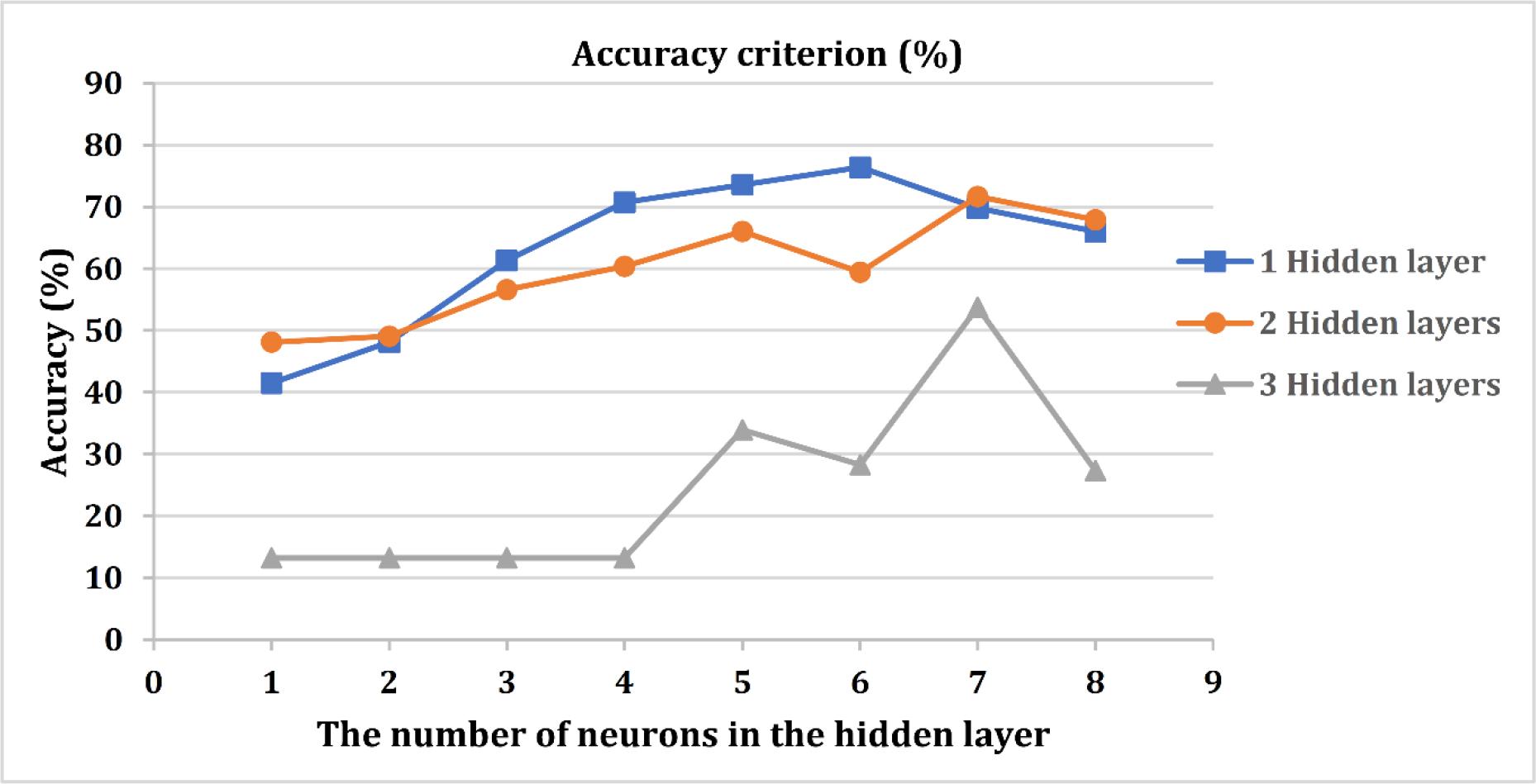
Accuracy of models with different numbers of neurons and hidden layers.
So, the best model identified had one hidden layer with six neurons. This model achieved the highest prediction accuracy among all models tested, with an accuracy of 76.42%. The error value for this model was 0.234, indicating a high level of accuracy in predicting the PDMs. This accuracy rate means that the ANN model correctly predicted the construction PDM for 76.42% of the test cases. This indicates the model’s effectiveness in generalising from training to unseen data.
The coefficients related to the connection of nodes in the hidden and output layer (weights) of the best model are listed in Tables 6 and 7, respectively. These weights indicate the importance and influence of each input variable on the model’s predictions. In other words, the model’s coefficients indicate the weight of each organisational characteristic in predicting the PDMs.
Connection coefficients of nodes in the hidden layer (best model)
| Variable | Node 1 | Node 2 | Node 3 | Node 4 | Node 5 | Node 6 |
|---|---|---|---|---|---|---|
| Managerial | 4.814 | 5.094 | 4.814 | –4.811 | –4.052 | –3.215 |
| Financial | 9.256 | 8.379 | 9.256 | –9.498 | –8.366 | –5.841 |
| Background | 5.696 | 3.822 | 5.696 | –4.698 | –3.133 | –2.998 |
| Optimisation | 2.981 | 2.587 | 2.981 | –2.511 | –2.684 | –1.871 |
| Energy efficiency | 0.581 | 0.510 | 0.581 | –0.940 | 0.019 | –0.506 |
| Bias | –7.437 | 2.136 | –7.437 | 1.524 | 9.801 | –3.991 |
Connection coefficients of nodes in the output layer (best model)
| Node | Output Node 1 | Output Node 2 | Output Node 3 | Output Node 4 | Output Node 5 | Output Node 6 |
|---|---|---|---|---|---|---|
| Node 1 | –1.454 | –1.818 | –1.712 | –2.103 | –2.073 | –4.525 |
| Node 2 | –3.075 | –3.961 | –2.565 | –11.451 | –10.190 | 2.895 |
| Node 3 | 2.199 | –4.315 | –0.647 | 0.256 | 2.389 | –1.400 |
| Node 4 | –2.566 | –2.195 | 0.493 | 6.947 | 16.573 | 9.320 |
| Node 5 | –3.351 | –3.045 | –1.206 | –2.245 | –5.482 | –3.947 |
| Node 6 | 9.765 | 10.638 | 2.272 | –3.172 | –14.231 | –23.596 |
| Threshold | –4.720 | –4.891 | –2.454 | –3.010 | –5.765 | –4.569 |
Thus, the best model was determined based on its high prediction accuracy and low error value. The model structure and the node connections were optimised to provide the best performance.
Figure 5 demonstrates the schematic of our final ANN model with one hidden layer and six neurons in the hidden layer. In the hidden layer, six neurons are shown along with a node called bias. The number of neurons in the input layer is equal to the number of predictor variables, i.e., five neurons along with bias. The number of neurons in the output layer is 12 neurons, equal to the number of PDMs.
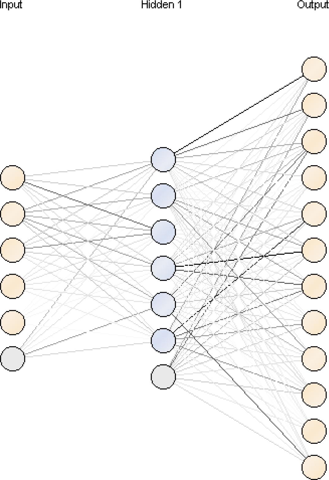
Schematic of the developed neural network model.
Other specifications of the ANN model are as follows:
The sigmoid activation function was used in the neural network model due to its effectiveness in handling binary classification problems and its ability to introduce non-linearity into the model.
The mean squared error (MSE) was employed as the error function to evaluate the model’s performance.
The method of calculating the nodes (for example, for one node in the hidden layer [Node1] and one node in the output layer [Class1]) is as follows:
According to the obtained neural network function, the type of PDM can be predicted based on the company’s information. The results of neural network classification accuracy are shown in Figure 6.
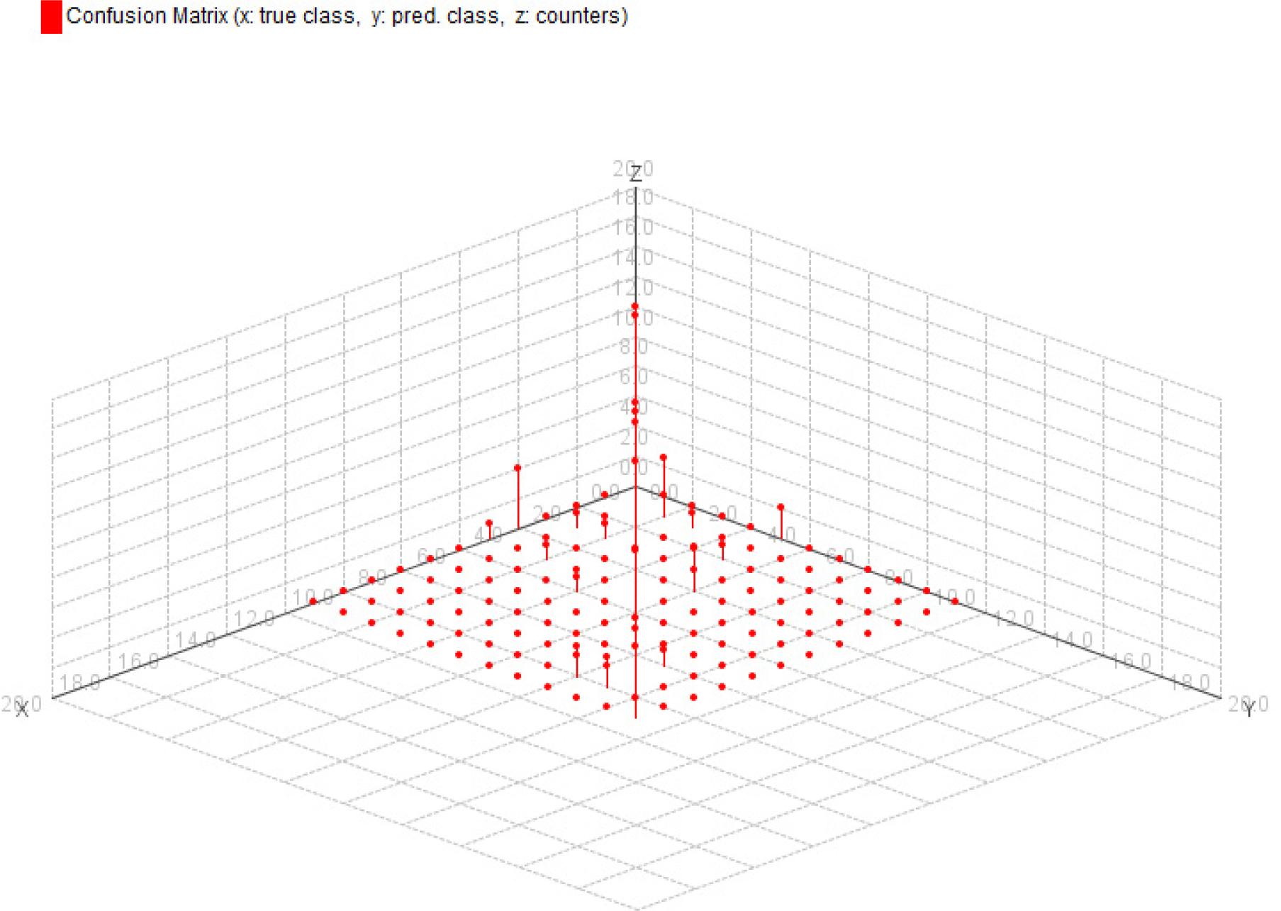
The result of data classification accuracy.
According to the results of the neural network model with one hidden layer and six neurons in the hidden layer with sigmoid activation function, it was observed that this model was able to correctly predict the construction the PDM with 76.42% accuracy.
To compare the accuracy results of the neural network model with the accuracy of other data mining models, the Naive Bayes, decision tree, random forest, and support vector machine (SVM) have been implemented on the data. The results are shown in Table 8. According to these results, the neural network algorithm identified in this research has shown the most accuracy among data mining algorithms.
Comparing the accuracy of data mining models
| Models | Accuracy criterion |
|---|---|
| Naive Bayes | 48.11 |
| Decision tree | 26.42 |
| Random forest | 13.21 |
| SVM | 13.21 |
| Selected neural network model | 76.42 |
SVM, support vector machine.
Additionally, common accuracy metrics such as the coefficient of determination (R2) and MAPE were utilised to assess the model’s precision and reliability. R2 measures the proportion of variance in the dependent variable that is predictable from the independent variables. It ranges from 0 to 1, with higher values indicating better model performance. MAPE measures the accuracy of the model as a percentage. It is calculated as the average absolute percentage error between the actual and predicted values. The comparison metrics are presented in Table 9.
Performance comparison of different models
| Model | R2 | MAPE (%) |
|---|---|---|
| ANN | 0.82 | 12.5 |
| Linear regression | 0.65 | 18.3 |
| Decision tree | 0.70 | 15.2 |
ANN, artificial neural network; MAPE, mean absolute percentage error.
The ANN model outperformed both the linear regression and decision tree in terms of both R2 and MAPE, indicating superior predictive accuracy and precision.
The research successfully achieved its goal of developing an accurate ANN model for predicting PDMs. The study highlighted the advantages of using ANN over traditional data mining models, emphasising its higher accuracy and ability to handle complex, non-linear relationships. The research also identified limitations such as the reliance on expert opinions and the need for large datasets for training the model.
This research developed an ANN model to predict the correct method of delivery of construction projects based on organisational characteristics. The ANN model demonstrated an accuracy of 76.42%, outperforming conventional data mining models such as the decision tree, random forest, and SVM. The research filled a gap in the literature by providing a robust predictive model that integrates organisational characteristics to determine the most suitable PDM. Previous studies have largely focussed on the performance outcomes of different PDMs without incorporating detailed organisational factors. Theoretically, this study contributes to the body of knowledge on project management and neural network applications by demonstrating the efficacy of ANN models in predicting PDMs. Managerially, the findings provide construction companies with a decision-support tool to select appropriate delivery methods, potentially improving project outcomes in terms of time, cost, and quality. While the study focussed on construction experts in the Mazandaran province, Iran, the methodology and insights are adaptable and can potentially be generalised to other regions with similar contexts. Additionally, the reliance on expert opinions in the Delphi method could introduce subjectivity. Future research could explore the application of the ANN model in different geographical regions and industry sectors to validate its generalisability. Additionally, integrating more advanced ANN architectures and additional variables, such as technological advancements and regulatory factors, could enhance the model’s predictive capability. Moreover, the findings of this research can contribute to BIM by providing a predictive framework for selecting PDMs that align with BIM’s goals of improving efficiency, reducing costs, and enhancing project quality.
The authors declare that they have no known competing financial interests or personal relationships that could have appeared to influence the work reported in this paper.