
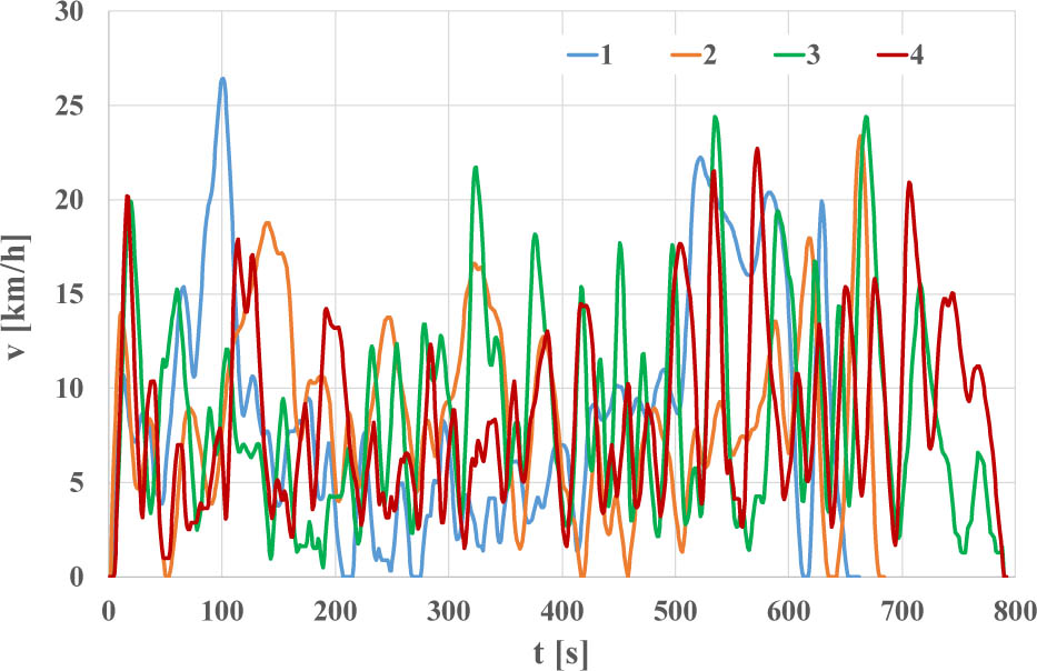
Figure 1.
Representations of the velocity process (v) in the CT test in the time domain (t)
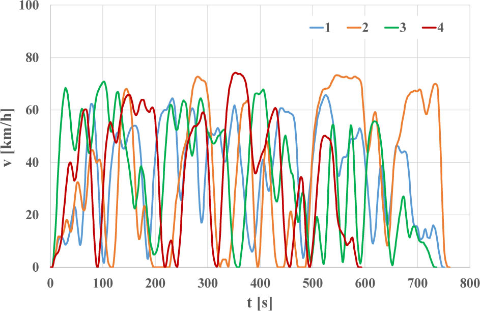
Figure 2.
Representations of the velocity process (v) in the UT test in the time domain (t)
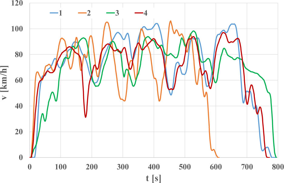
Figure 3.
Representations of the velocity process (v) in the RT test in the time domain (t)
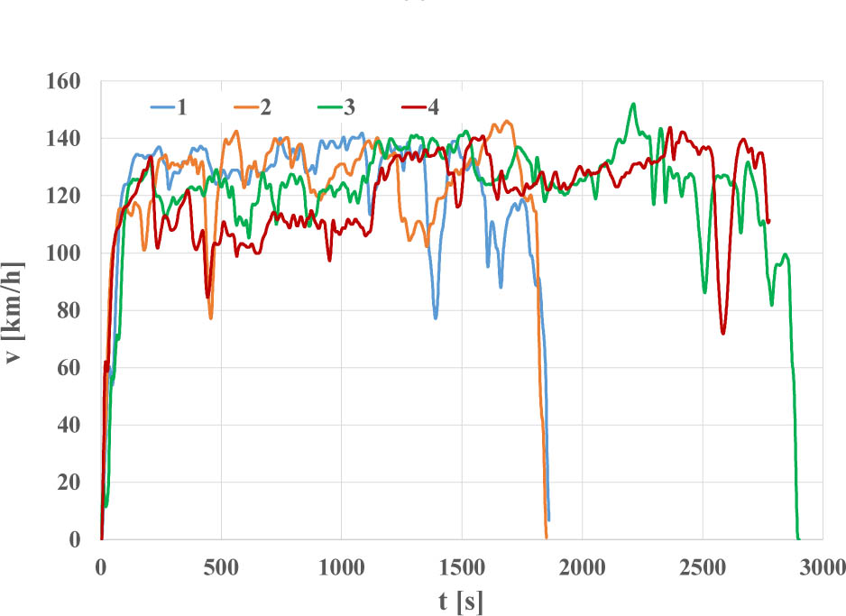
Figure 4.
Representations of the velocity process (v) in the HT test in the time domain (t)
Table 1.
Statistical zero-dimensional characteristics of the CT test process
| CT | ||||
|---|---|---|---|---|
| 1 | 2 | 3 | 4 | |
| AV | 8.6 | 8.5 | 8.5 | 8.4 |
| M | 7.6 | 8.0 | 7.3 | 7.4 |
| D | 6.33 | 4.86 | 5.37 | 4.75 |
| K | −0.213 | −0.145 | −0.025 | −0.169 |
| S | 0.784 | 0.419 | 0.748 | 0.687 |
| R | 26.4 | 23.4 | 24.4 | 22.7 |
| Min | 0.0 | 0.0 | 0.0 | 0.0 |
| Max | 26.4 | 23.4 | 24.4 | 22.7 |
| W | 0.737 | 0.571 | 0.629 | 0.563 |
| Q1 | 3.9 | 5.1 | 4.3 | 4.6 |
| Q3 | 10.9 | 11.6 | 11.9 | 11.6 |
| RQ | 2.8 | 2.3 | 2.8 | 2.5 |
| DQ | 1.4 | 1.1 | 1.4 | 1.2 |
| WQ | 0.1813 | 0.1437 | 0.1924 | 0.1694 |
Table 2.
Statistical zero-dimensional characteristics of the UT test process
| UT | ||||
|---|---|---|---|---|
| 1 | 2 | 3 | 4 | |
| AV | 36.0 | 36.0 | 36.0 | 36.0 |
| M | 40.5 | 37.3 | 39.7 | 39.9 |
| D | 18.73 | 26.22 | 21.42 | 23.17 |
| K | −1.232 | −1.525 | −1.332 | −1.358 |
| S | −0.285 | −0.009 | −0.181 | −0.180 |
| R | 65.7 | 73.3 | 70.8 | 74.2 |
| Min | 0.0 | 0.0 | 0.0 | 0.0 |
| Max | 65.7 | 73.3 | 70.8 | 74.2 |
| W | 0.520 | 0.728 | 0.595 | 0.643 |
| Q1 | 17.4 | 10.9 | 15.6 | 11.3 |
| Q3 | 51.4 | 62.9 | 54.0 | 56.3 |
| RQ | 3.0 | 5.8 | 3.5 | 5.0 |
| DQ | 1.5 | 2.9 | 1.7 | 2.5 |
| WQ | 0.0366 | 0.0771 | 0.0437 | 0.0624 |
Table 3.
Statistical zero-dimensional characteristics of the RT test process
| RT | ||||
|---|---|---|---|---|
| 1 | 2 | 3 | 4 | |
| AV | 70.7 | 70.6 | 69.6 | 70.7 |
| M | 76.4 | 72.3 | 76.1 | 77.3 |
| D | 28.09 | 24.43 | 21.46 | 21.40 |
| K | 0.662 | 1.346 | 1.948 | 2.000 |
| S | −1.170 | −1.181 | −1.440 | −1.445 |
| R | 104.1 | 106.0 | 98.2 | 97.0 |
| Min | 0.0 | 0.0 | 0.0 | 0.0 |
| Max | 104.1 | 106.0 | 98.2 | 97.0 |
| W | 0.397 | 0.346 | 0.308 | 0.303 |
| Q1 | 59.1 | 61.4 | 61.3 | 60.8 |
| Q3 | 92.5 | 89.8 | 84.8 | 86.0 |
| RQ | 1.6 | 1.5 | 1.4 | 1.4 |
| DQ | 0.8 | 0.7 | 0.7 | 0.7 |
| WQ | 0.0102 | 0.0101 | 0.0091 | 0.0091 |
Table 4.
Statistical zero-dimensional characteristics of the HT test process
| HT | ||||
|---|---|---|---|---|
| 1 | 2 | 3 | 4 | |
| AV | 122.5 | 121.4 | 121.4 | 117.9 |
| M | 129.9 | 124.7 | 124.7 | 122.2 |
| D | 22.64 | 20.83 | 20.83 | 19.00 |
| K | 8.784 | 12.977 | 12.977 | 10.287 |
| S | −2.745 | −3.182 | −3.182 | −2.393 |
| R | 141.8 | 152.0 | 152.0 | 143.8 |
| Min | 0.0 | 0.0 | 0.0 | 0.0 |
| Max | 141.8 | 152.0 | 152.0 | 143.8 |
| W | 0.185 | 0.172 | 0.172 | 0.161 |
| Q1 | 120.4 | 119.7 | 119.7 | 108.9 |
| Q3 | 135.3 | 131.5 | 131.5 | 131.3 |
| RQ | 1.1 | 1.1 | 1.1 | 1.2 |
| DQ | 0.6 | 0.5 | 0.5 | 0.6 |
| WQ | 0.0043 | 0.0044 | 0.0044 | 0.0049 |
[i] Note: AV: average value; M: median (second quartile Q2); D: standard deviation; DQ: quartile deviation; K: kurtosis; S: skewness; Min: minimum value; Max: maximum value; Q1: first quartile; Q3: third quartile; R: range; RQ: interquartile range; W: coefficient of variation; WQ: quartile coefficient of variation.
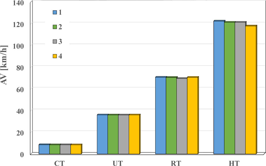
Figure 5.
Average value (AV) of the CT, UT, RT and HT velocity process representation
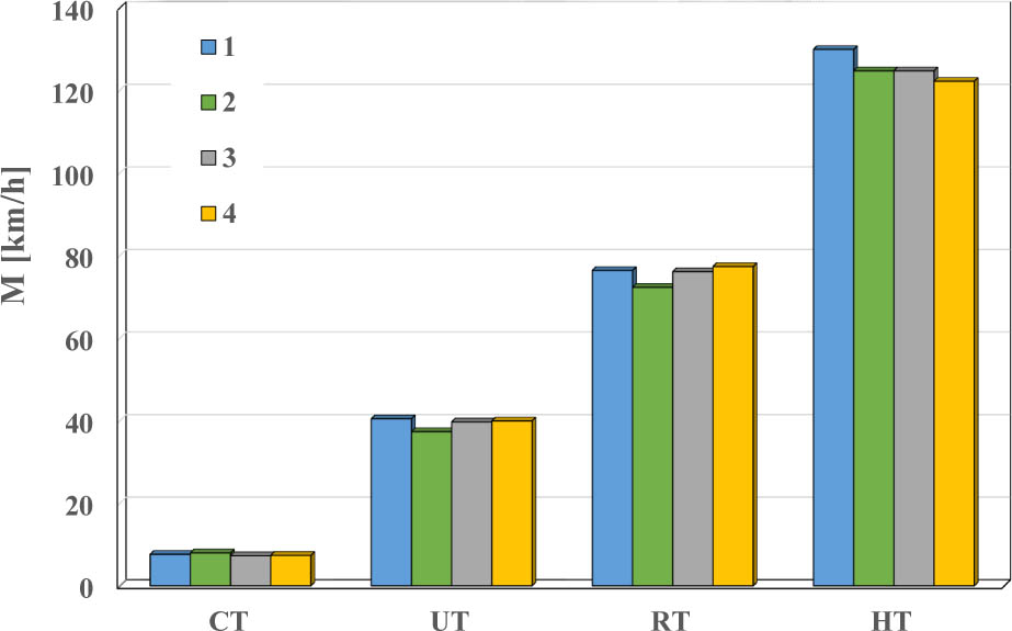
Figure 6.
Median (M) of the CT, UT, RT and HT velocity process representation
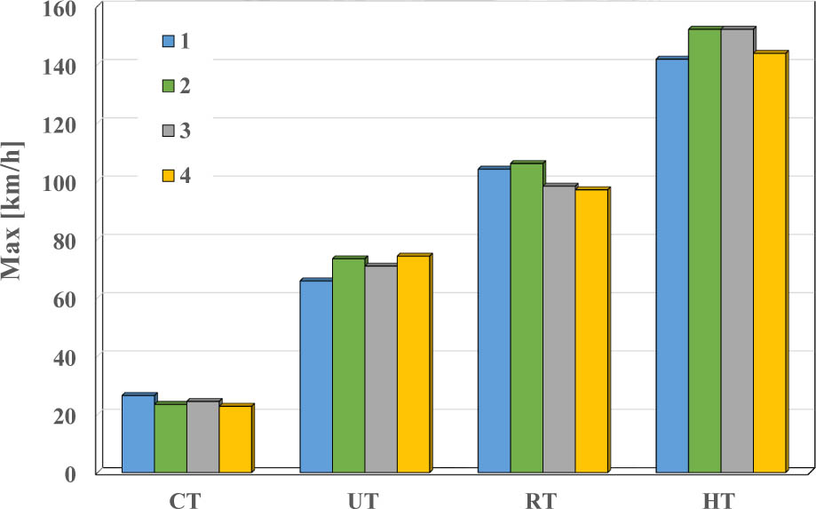
Figure 7.
Maximum value (Max) of the CT, UT, RT and HT velocity process representation
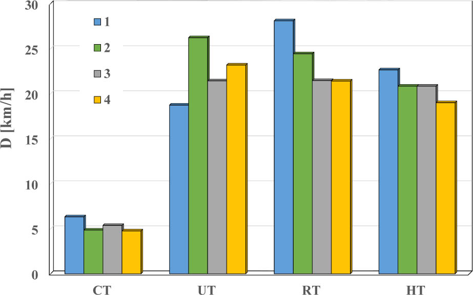
Figure 8.
Standard deviation (D) of the CT, UT, RT and HT velocity process representations
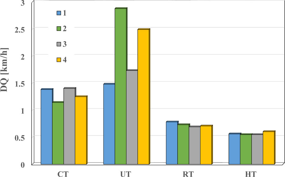
Figure 9.
Quartile deviation (DQ) of the CT, UT, RT and HT velocity process representations
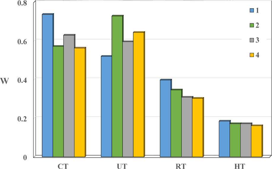
Figure 10.
Coefficient of variation (W) of the CT, UT, RT and HT velocity process representations
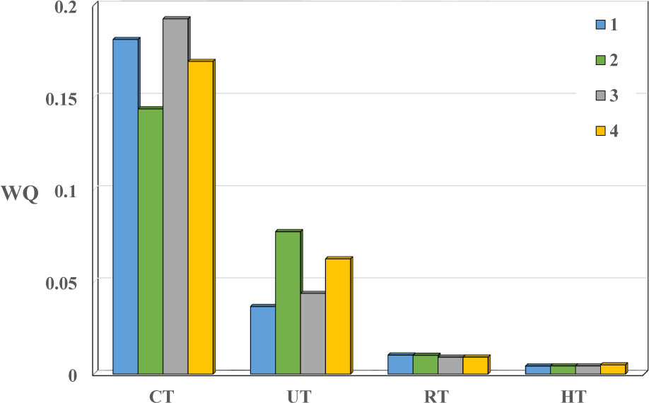
Figure 11.
Quartile coefficient of variation (WQ) of the CT, UT, RT and HT velocity process representations
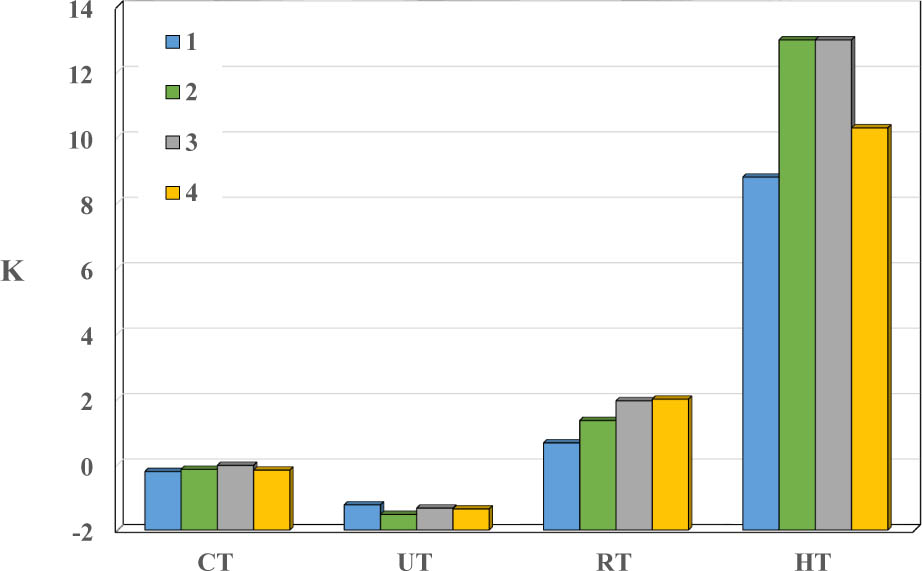
Figure 12.
Kurtosis (K) of the CT, UT, RT and HT velocity process representations
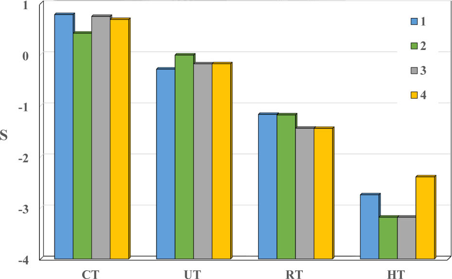
Figure 13.
Skewness (S) of the CT, UT, RT and HT velocity process representation
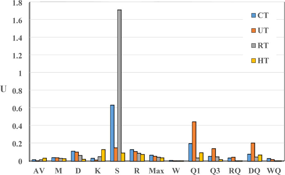
Figure 14.
The uniqueness (U) of the zero-dimensional characteristics of the CT, UT, RT and HT velocity process representations
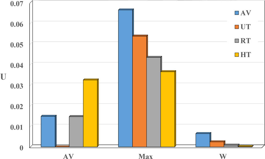
Figure 15.
The uniqueness (U) of the average value, maximum value and coefficient of variation of the CT, UT, RT and HT velocity process representations
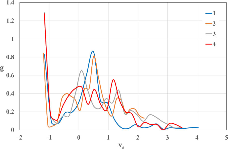
Figure 16.
Probability density (g) of the CT process representations depending on the standardized velocity (vs)
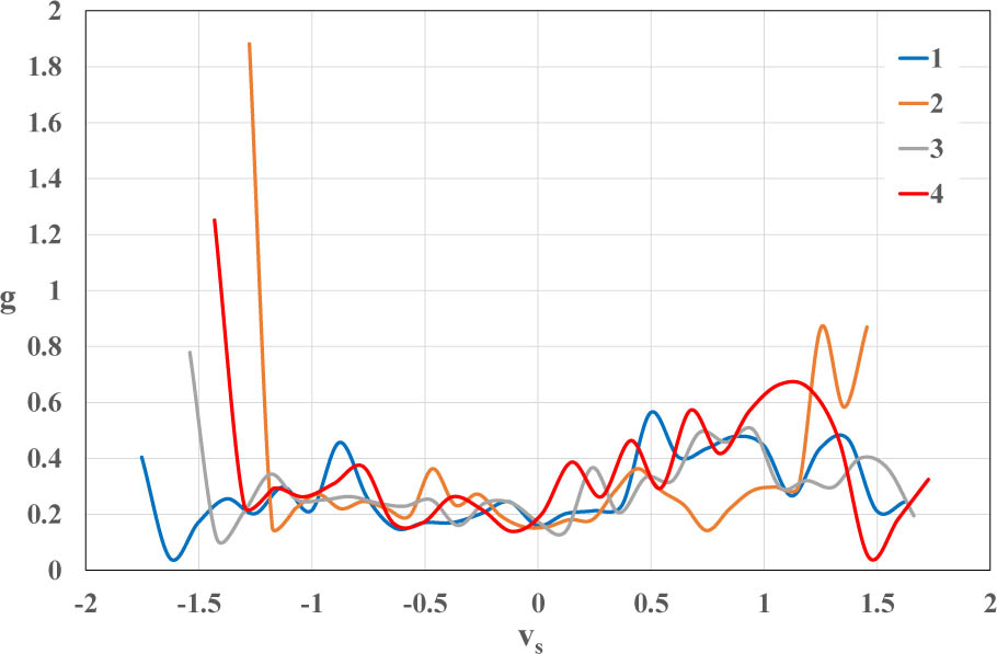
Figure 17.
Probability density (g) of the UT process representations depending on the standardized velocity (vs)
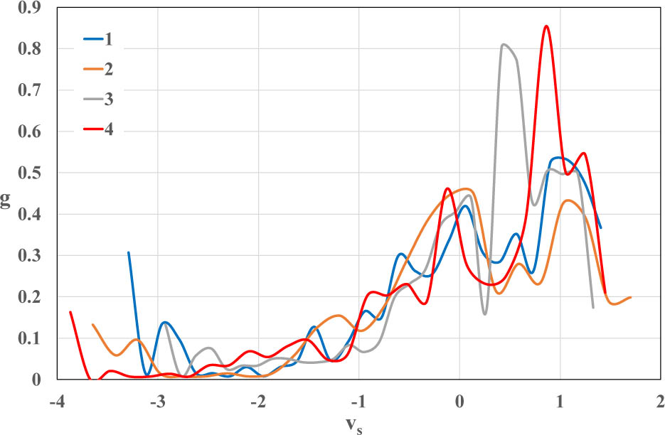
Figure 18.
Probability density (g) of the RT process representations depending on the standardized velocity (vs)
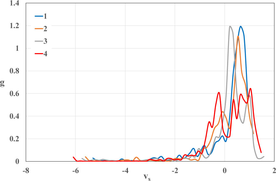
Figure 19.
Probability density (g) of the HT process representations depending on the standardized velocity (vs)
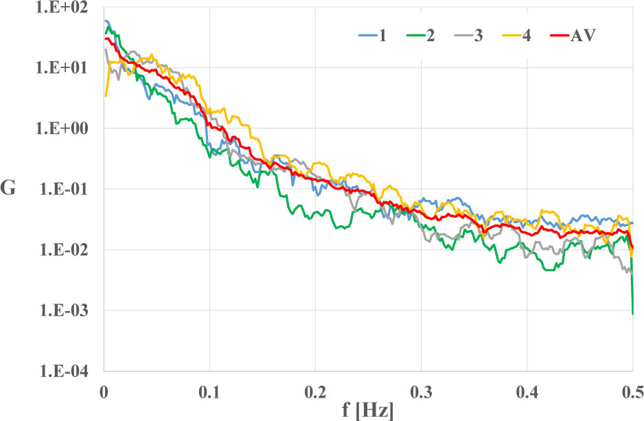
Figure 20.
Power spectral density of the CT process representations and the average value (AV) for all representations in the frequency domain (f)
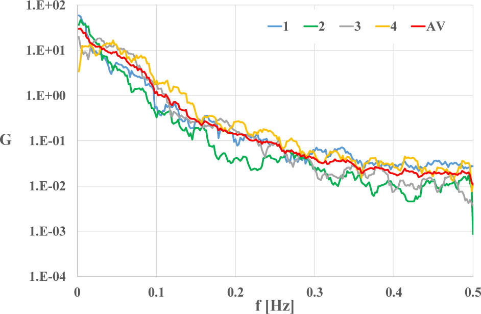
Figure 21.
Power spectral density of the UT process representations and the average value (AV) for all representations in the frequency domain (f)
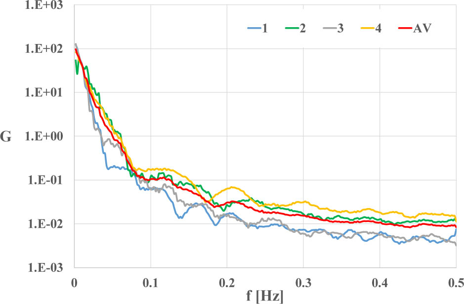
Figure 22.
Power spectral density of the RT process representations and the average value (AV) for all representations in the frequency domain (f)
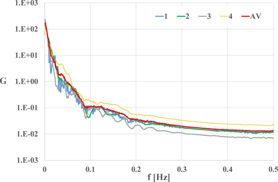
Figure 23.
Power spectral density of the HT process representations and the average value (AV) for all representations in the frequency domain (f)
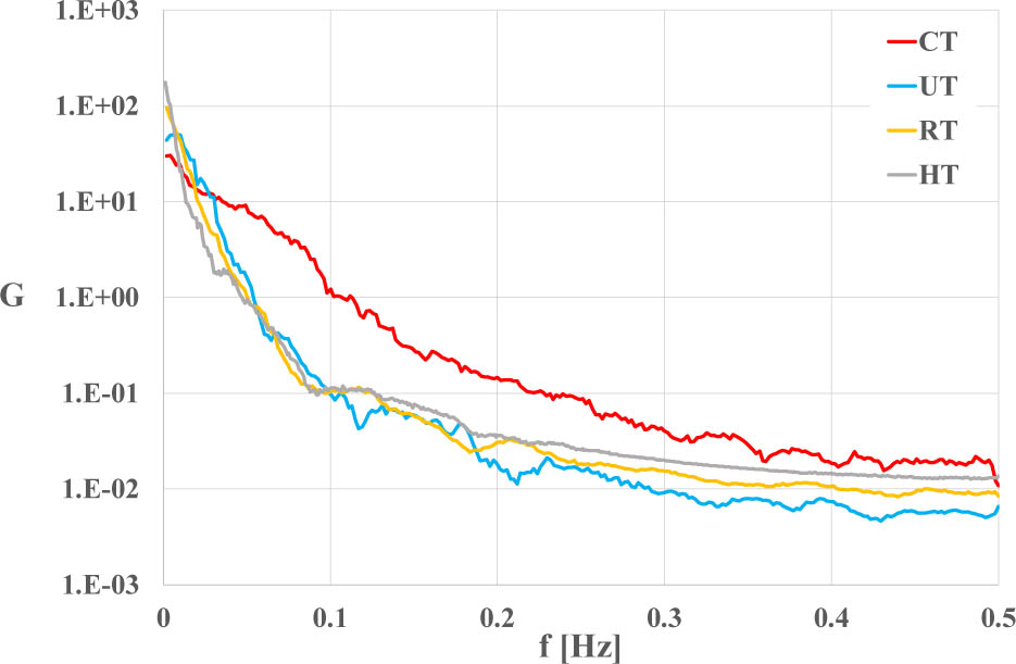
Figure 24.
The joint power spectral density of the CT, UT, RT and HT process representations in the frequency domain (f)