
1. INTRODUCTION
The properties of objects are determined by their inherent features, by the states in which they exist, and by the conditions of their operation. In the case of road vehicles, operational properties are related primarily to:
– energy consumption,
– environmental impact,
– reliability, durability and operational quality, in particular maintenance [Andrych-Zalewska et al. 2022; Andrych-Zalewska et al. 2021; Chłopek et al. July 2013; Kurtyka, Pielecha 2019].
Energy consumption by road vehicles depends on their overall efficiency and the operating conditions. For road vehicles powered by internal combustion engines, energy consumption is determined by fuel consumption.
In general, the term ‘pollution’ refers to an impact on the environment that significantly adversely changes its properties. Environmental pollution may be classified as follows:
– substantial pollution—introducing substances harmful to the environment,
– energetic pollution—concerning primarily electromagnetic radiation and noise,
– informational pollution [Bebkiewicz et al. 2021; Bebkiewicz et al. Sept. 2021].
In common understanding, the term pollution most often means substantial pollution, which are divided into:
– those harmful to organisms, commonly called toxic,
– those causing adverse changes in environmental properties, primarily substances contributing to the intensification of the greenhouse effect [Bebkiewicz et al. 2021; Bebkiewicz et al. Sept. 2021].
In the case of the impact of road vehicles on the environment, the greatest attention is currently paid to the emission of substantial pollutants and noise [AVL 2016; DieselNet; WES 2021]. The primary source of both type of emission is the combustion engine in the vehicles. In addition, the sources of particulate matter emission are tribological pairs in road transport, primarily the braking system, clutches and tyres of road wheels interacting with the road surface [Bebkiewicz et al. 2021; Bebkiewicz et al. Sept. 2021; EEA/EMEP 2023].
The operating state of road vehicles and, consequently, their internal combustion engines depends on vehicle velocity courses and the conditions of vehicle use [Andrych-Zalewska et al. 2022; Andrych-Zalewska et al. 2021; Bebkiewicz et al. 2021; Bebkiewicz et al. Sept. 2021; Chłopek et al. 2014; Chłopek et al. 2013; Chłopek et al. July 2013; Chłopek 2014]. For this reason, procedures for testing vehicle operational properties engage driving tests, as vehicle velocity courses are treated as velocity processes. In real-world traffic, vehicle velocity is inherently non-repeatable due to driver behaviour, traffic interactions, infrastructure characteristics and environmental conditions. As a result, velocity courses exhibit stochastic properties, and their statistical characteristics cannot be fully captured by deterministic driving cycles. This motivates the need for research into stochastic representations of driving processes, which may provide a more realistic basis for evaluating vehicle operational and environmental performance.
In mathematical terms, a process represents quantities defined over a normed space [Conway 1990; Weisstein 2025]. A normed space is a linear space [Andrych-Zalewska et al. 2021; DieselNet] in which the concept of a norm is defined as a generalisation of the concept of the length (modulus) of a vector in Euclidean space [Conway 1990; Weisstein 2025].
The domain in which a process is defined most often includes:
– time or a monotonic function of time (process–time function, time series),
– area of space (process–field).
Process analyses are typically conducted in the following domains:
– time (e.g. autocorrelation function, cross-correlation function, statistical characteristics) [Bendat, Piersol 2010; Box et al. 1978, Lane et al. 2003; McClave, Sincich 2012; Otnes, Enochson 1978; Ralston, Rabinowitz 2001; Utts, Heckard 2014],
– frequency (e.g. power spectral density) [Bendat, Piersol 2010; Conway 1990; Ralston, Rabinowitz 2001],
– process value (e.g. histogram, probability density) [Bendat, Piersol 2010; Ioannidis 2003; Otnes, Enochson 1978; Ralston, Rabinowitz 2001].
An important classification of processes concerns their determinacy, which is particularly relevant in complex studies such as vehicle properties evaluation. This classification includes:
– causal (or deterministic) processes,
– random (or stochastic) processes [Bendat, Piersol 2010; Chłopek et al. 2014; Chłopek et al. 2013; Chłopek et al. July 2013; Chłopek 2016; Otnes, Enochson 1978; Papoulis, Pillai 2002; Parzen 2015].
The concept of causal processes is essentially theoretical, as in reality there is always a certain degree of uncertainty and non-repeatability in testing conditions.
A typical example of a velocity process treated as a random process by definition is the RDE (Real Driving Emissions) test [Andrych-Zalewska et al. 2022; Andrych-Zalewska et al. 2021; AVL 2016; Kurtyka, Pielecha 2019; WES 2021], which is conducted under real-world driving conditions. The RDE test is subject only to general procedural constraints [AVL 2016; WES 2021].
Random driving velocity processes may also be represented as sets of process realizations-recorded vehicle velocity courses under comparable traffic conditions (primarily characterized by the mean value, standard deviation, and coefficient of variation of the process realizations) [Chłopek et al. 2014; Chłopek et al. 2013; Chłopek et al. July 2013; Papoulis, Pillai 2002; Parzen 2015].
Another important classification concerns the dependence of processes on time. Processes that are constant in time are static, while those that change in time are dynamic. This division is of great importance in relation to the properties of combustion engines when considering pollutant emissions. These properties may vary considerably depending on whether the engine operating states are static or dynamic, as the engine operating states are determined by vehicle velocity processes [Andrych-Zalewska et al. 2022; Andrych-Zalewska et al. 2021; Chłopek 2014].
The stability of process characteristics in the argument domain is associated with the problem of stationarity [Markov 1906; Papoulis, Pillai 2002; Parzen 2015].
Driving tests for examining vehicle properties are based on vehicle velocity processes with properties corresponding to the actual use of vehicles [André 2004; Andrych-Zalewska et al. 2022; Andrych-Zalewska et al. 2021; AVL 2016; Bebkiewicz et al. 2021; Bebkiewicz et al. Sept. 2021; BUWAL; Chłopek et al. 2014; Chłopek et al. 2013; Chłopek et al. July 2013].
The methods for creating driving tests include [André 2004; Chłopek et al. 2014; Chłopek et al. 2013; Chłopek et al. July 2013; DieselNet; UITP]:
– methods based on recorded vehicle velocity courses in accordance with the conditions of vehicle actual use-accurate simulation in the time domain with the possibility of synthesizing the test using representative registered vehicle courses (e.g. using the Monte Carlo method [Chłopek 2009; Fishman 1996; Metropolis, Ulam 1949]), FTP 75, WLTC),
– methods based on the synthesis of vehicle velocity courses according to a predefined velocity course and identification of test parameters (e.g. NEDC),
– methods based on the similarity of characteristics in the frequency domain [Chłopek 2016].
Although numerous studies have examined vehicle operating conditions, pollutant emissions and the construction of driving tests, the existing literature remains fragmented in several important respects. Prior research has predominantly focused on deterministic driving cycles which – despite their widespread regulatory use – do not capture the stochastic and non-repeatable nature of real driving conditions. Studies on real driving emissions acknowledge this variability, yet they typically analyse individual velocity traces rather than treating driving behaviour as a stochastic process with definable statistical properties.
Moreover, while many works discuss the environmental impacts of vehicle operation, they rarely link these impacts directly to the mathematical characteristics of driving velocity processes. The relationship between process dynamics (such as variability or spectral properties) and operational or environmental outcomes, including fuel consumption and pollutant emissions, remains insufficiently explored. Existing methodologies for constructing driving tests often prioritise representativeness in either the time or frequency domain, but few studies assess whether stochastic models can provide stable and generalisable representations of real driving behaviour.
These gaps motivate the present study, which aims to analyse driving velocity explicitly as a stochastic process and to investigate how its statistical and dynamic properties relate to vehicle operational behaviour and potential environmental impacts. In particular, the study seeks to determine whether stochastic velocity models can serve as reliable and statistically robust representations of real-world driving conditions, and how their dynamic characteristics may influence fuel consumption and pollutant emissions.
ENVIRONMENTAL CONTEXT AND RELEVANCE
Driving velocity processes directly determine the operating states of vehicle powertrains, including the frequency and intensity of transient engine conditions such as acceleration, deceleration and load changes. These transient states are known to significantly influence fuel consumption and the emission of pollutants such as nitrogen oxides, carbon dioxide and particulate matter.
Highly dynamic driving, characteristic of urban traffic, typically leads to increased fuel demand, more frequent enrichment phases, higher exhaust temperatures and intensified brake and tyre wear, all of which contribute to substantial and energetic pollution. Conversely, low-dynamic fast-road driving is associated with more stable engine operation but increased fuel consumption, affecting carbon dioxide emissions.
By analysing stochastic velocity processes, this study provides insight into the variability of real-world driving conditions and their potential environmental consequences. Understanding these relationships is essential for improving emission modelling, developing representative driving tests and supporting environmental policy and vehicle design.
STOCHASTIC DRIVING TESTS
As part of our own work [Chłopek et al. 2014; Chłopek et al. 2013; Chłopek et al. July 2013], stochastic models of the passenger car velocity process were developed in the following traffic conditions: urban driving congestion, urban driving without congestion, extra-urban driving and fast road driving (on highways and expressways) [Andrych-Zalewska et al. 2022; Andrych-Zalewska et al. 2021; EEA/EMEP 2023]. Based on the results of empirical studies, stochastic tests were determined in the form of sets of velocity process realizations in model traffic conditions. These tests were determined by recording the velocity of the vehicle in comparable traffic conditions. The recorded signals were processed, primarily by low-pass filtering to reduce the high-frequency noise content of the signals. For this purpose, the Savitzky-Golay filter with a five-point approximation by third-degree polynomial was used [Savitzky, Golay 1964].
All recorded velocity courses were analysed for statistical features-zero-dimensional statistical characteristics [Bendat, Piersol 2010; Box et al. 1978; Lane et al. 2003; Utts, Heckard 2014], primarily: mean value, standard deviation and coefficient of variation. It was postulated that the courses that had similar values of the analysed statistical features should be treated as representations of velocity processes.
In this study, representative driving velocity processes were selected through a systematic procedure applied to multiple real-world velocity course recordings obtained under comparable traffic and environmental conditions. The aim of this procedure was to identify process realizations that reliably reflect the statistical properties of typical vehicle operation within each analysed driving context.
The selection was performed in two stages. In the first stage, all recorded velocity courses were evaluated using basic statistical descriptors, including mean velocity, standard deviation and coefficient of variation. These descriptors were used to assess the similarity of individual realizations and to exclude outliers resulting from atypical traffic disturbances, irregular driver behaviour or measurement artefacts. Only realizations whose statistical characteristics fell within an acceptable deviation range from the sample median were retained for further analysis.
In the second stage, the retained realizations were compared using a non-repeatability threshold, defined as the maximum allowable relative deviation of key statistical parameters between realizations. This threshold ensured that the selected processes exhibited sufficient internal consistency while still reflecting the inherent stochasticity of real-world driving. The threshold value was determined based on preliminary analyses and supported by findings from previous studies on the variability of driving processes. These studies indicate that excessively strict thresholds suppress natural variability, whereas overly permissive thresholds reduce representativeness. The adopted value therefore balances these considerations and ensures that the selected processes are both statistically stable and realistic.
The final set of representative processes consists of realizations that meet both criteria: statistical similarity to the central tendency of the dataset and compliance with the non-repeatability threshold. These representative processes form the basis for subsequent analyses of dynamic properties, spectral characteristics and their potential implications for vehicle operational behaviour and environmental impacts.
Figures 1–4 show example representations of velocity processes modelling vehicle movement in typical traffic conditions: urban driving with congestion (CT), urban driving without congestion (UT), extra-urban (rural) driving (RT) and fast road driving (on highways and expressways) (HT).
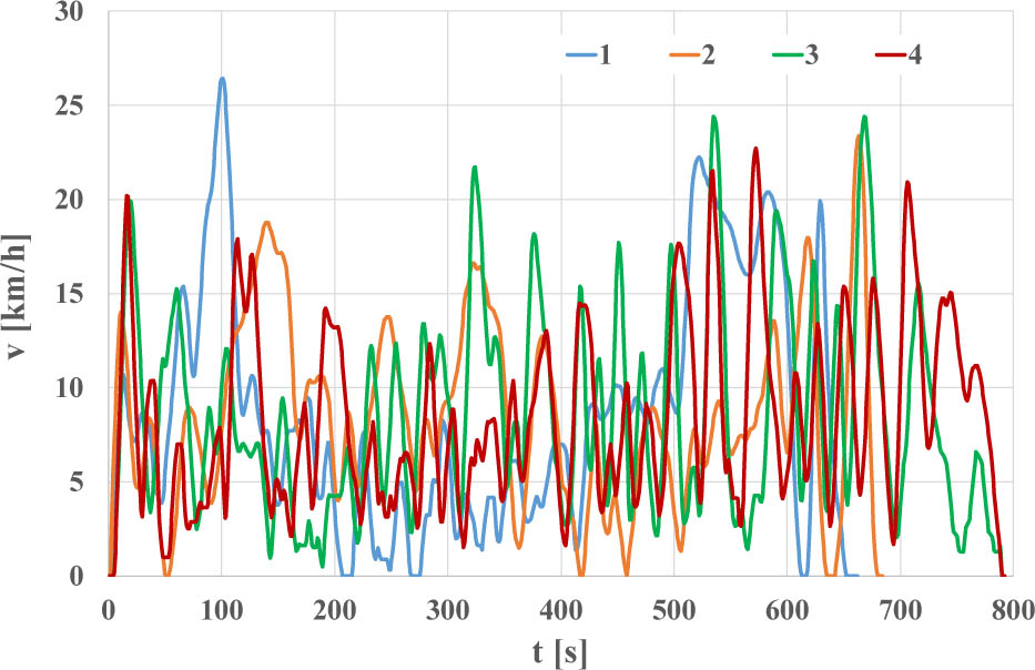
Figure 1.
Representations of the velocity process (v) in the CT test in the time domain (t)
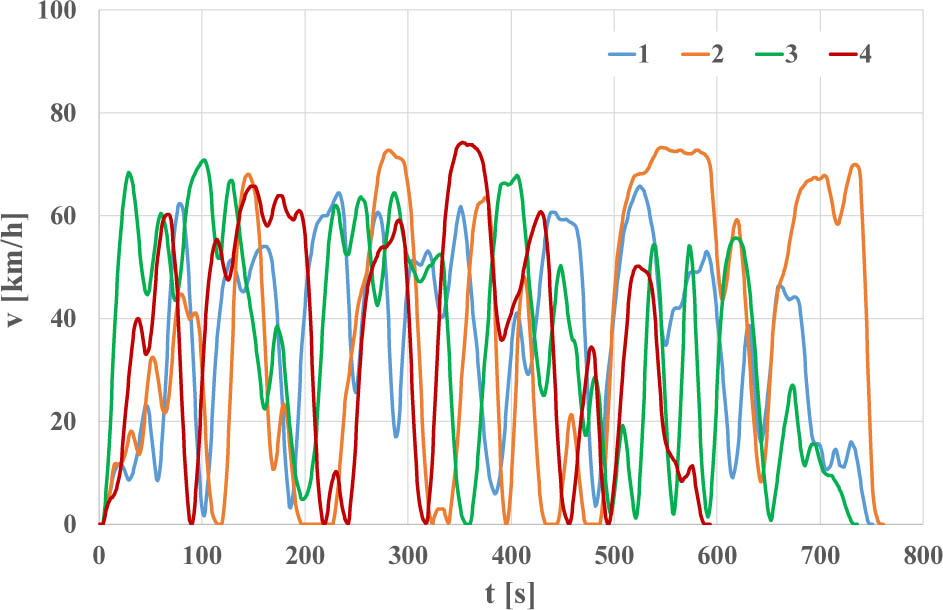
Figure 2.
Representations of the velocity process (v) in the UT test in the time domain (t)
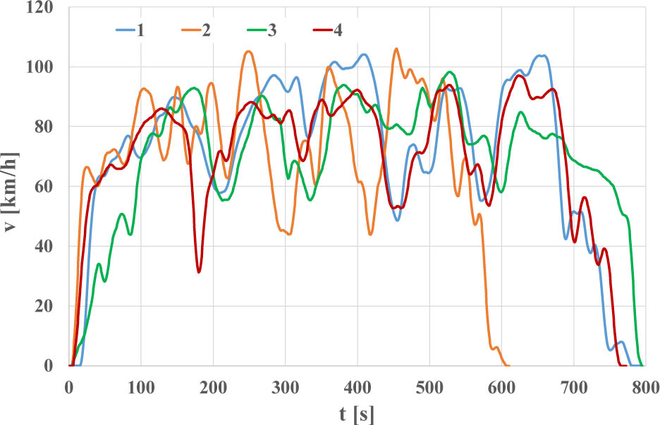
Figure 3.
Representations of the velocity process (v) in the RT test in the time domain (t)
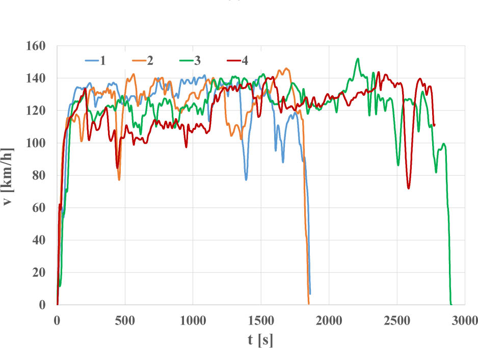
Figure 4.
Representations of the velocity process (v) in the HT test in the time domain (t)
ANALYSIS OF STOCHASTIC DRIVING TESTS
The following zero-dimensional statistical characteristics of the studied tests were determined, separately for each process representation, as well as for all representations in total [Bendat, Piersol 2010; Box et al. 1978; Lane et al. 2003, Utts, Heckard 2014].
The calculated values of the above zero-dimensional statistical characteristics are presented in tables 1–4.
Table 1.
Statistical zero-dimensional characteristics of the CT test process
| CT | ||||
|---|---|---|---|---|
| 1 | 2 | 3 | 4 | |
| AV | 8.6 | 8.5 | 8.5 | 8.4 |
| M | 7.6 | 8.0 | 7.3 | 7.4 |
| D | 6.33 | 4.86 | 5.37 | 4.75 |
| K | −0.213 | −0.145 | −0.025 | −0.169 |
| S | 0.784 | 0.419 | 0.748 | 0.687 |
| R | 26.4 | 23.4 | 24.4 | 22.7 |
| Min | 0.0 | 0.0 | 0.0 | 0.0 |
| Max | 26.4 | 23.4 | 24.4 | 22.7 |
| W | 0.737 | 0.571 | 0.629 | 0.563 |
| Q1 | 3.9 | 5.1 | 4.3 | 4.6 |
| Q3 | 10.9 | 11.6 | 11.9 | 11.6 |
| RQ | 2.8 | 2.3 | 2.8 | 2.5 |
| DQ | 1.4 | 1.1 | 1.4 | 1.2 |
| WQ | 0.1813 | 0.1437 | 0.1924 | 0.1694 |
Table 2.
Statistical zero-dimensional characteristics of the UT test process
| UT | ||||
|---|---|---|---|---|
| 1 | 2 | 3 | 4 | |
| AV | 36.0 | 36.0 | 36.0 | 36.0 |
| M | 40.5 | 37.3 | 39.7 | 39.9 |
| D | 18.73 | 26.22 | 21.42 | 23.17 |
| K | −1.232 | −1.525 | −1.332 | −1.358 |
| S | −0.285 | −0.009 | −0.181 | −0.180 |
| R | 65.7 | 73.3 | 70.8 | 74.2 |
| Min | 0.0 | 0.0 | 0.0 | 0.0 |
| Max | 65.7 | 73.3 | 70.8 | 74.2 |
| W | 0.520 | 0.728 | 0.595 | 0.643 |
| Q1 | 17.4 | 10.9 | 15.6 | 11.3 |
| Q3 | 51.4 | 62.9 | 54.0 | 56.3 |
| RQ | 3.0 | 5.8 | 3.5 | 5.0 |
| DQ | 1.5 | 2.9 | 1.7 | 2.5 |
| WQ | 0.0366 | 0.0771 | 0.0437 | 0.0624 |
Table 3.
Statistical zero-dimensional characteristics of the RT test process
| RT | ||||
|---|---|---|---|---|
| 1 | 2 | 3 | 4 | |
| AV | 70.7 | 70.6 | 69.6 | 70.7 |
| M | 76.4 | 72.3 | 76.1 | 77.3 |
| D | 28.09 | 24.43 | 21.46 | 21.40 |
| K | 0.662 | 1.346 | 1.948 | 2.000 |
| S | −1.170 | −1.181 | −1.440 | −1.445 |
| R | 104.1 | 106.0 | 98.2 | 97.0 |
| Min | 0.0 | 0.0 | 0.0 | 0.0 |
| Max | 104.1 | 106.0 | 98.2 | 97.0 |
| W | 0.397 | 0.346 | 0.308 | 0.303 |
| Q1 | 59.1 | 61.4 | 61.3 | 60.8 |
| Q3 | 92.5 | 89.8 | 84.8 | 86.0 |
| RQ | 1.6 | 1.5 | 1.4 | 1.4 |
| DQ | 0.8 | 0.7 | 0.7 | 0.7 |
| WQ | 0.0102 | 0.0101 | 0.0091 | 0.0091 |
Table 4.
Statistical zero-dimensional characteristics of the HT test process
| HT | ||||
|---|---|---|---|---|
| 1 | 2 | 3 | 4 | |
| AV | 122.5 | 121.4 | 121.4 | 117.9 |
| M | 129.9 | 124.7 | 124.7 | 122.2 |
| D | 22.64 | 20.83 | 20.83 | 19.00 |
| K | 8.784 | 12.977 | 12.977 | 10.287 |
| S | −2.745 | −3.182 | −3.182 | −2.393 |
| R | 141.8 | 152.0 | 152.0 | 143.8 |
| Min | 0.0 | 0.0 | 0.0 | 0.0 |
| Max | 141.8 | 152.0 | 152.0 | 143.8 |
| W | 0.185 | 0.172 | 0.172 | 0.161 |
| Q1 | 120.4 | 119.7 | 119.7 | 108.9 |
| Q3 | 135.3 | 131.5 | 131.5 | 131.3 |
| RQ | 1.1 | 1.1 | 1.1 | 1.2 |
| DQ | 0.6 | 0.5 | 0.5 | 0.6 |
| WQ | 0.0043 | 0.0044 | 0.0044 | 0.0049 |
[i] Note: AV: average value; M: median (second quartile Q2); D: standard deviation; DQ: quartile deviation; K: kurtosis; S: skewness; Min: minimum value; Max: maximum value; Q1: first quartile; Q3: third quartile; R: range; RQ: interquartile range; W: coefficient of variation; WQ: quartile coefficient of variation.
Tables 1–4 show that the mean values and maximum values within each traffic category are highly consistent, confirming the statistical coherence of the selected representations. The coefficients of variation and quartile coefficients of variation reveal substantial differences in dynamic behaviour between traffic conditions. Urban driving (CT, UT) exhibits high variability, which is associated with frequent transient engine states and therefore higher potential emissions. Fast-road driving (HT) shows low variability, indicating more stable engine operation but higher aerodynamic loads.
Figures 5–13 present zero-dimensional statistical characteristics of the investigated velocity processes for all process representations.
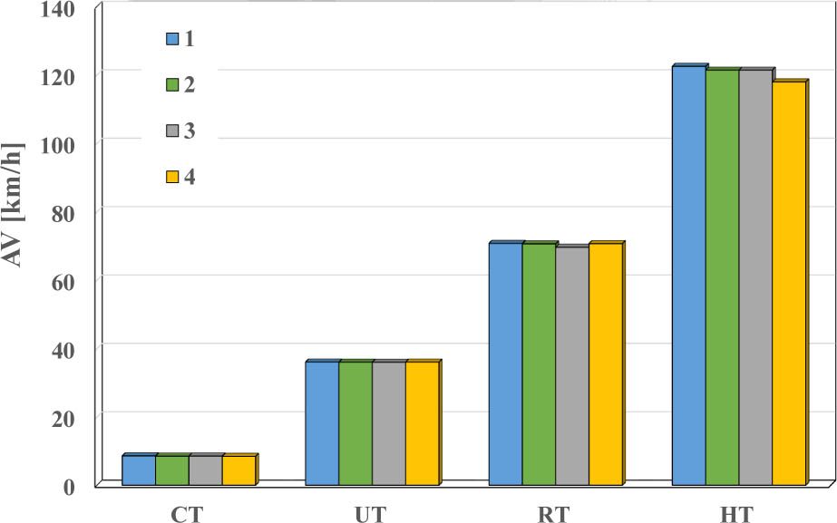
Figure 5.
Average value (AV) of the CT, UT, RT and HT velocity process representation
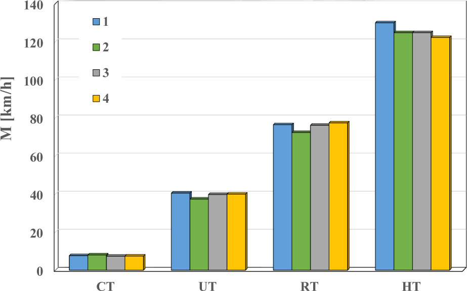
Figure 6.
Median (M) of the CT, UT, RT and HT velocity process representation
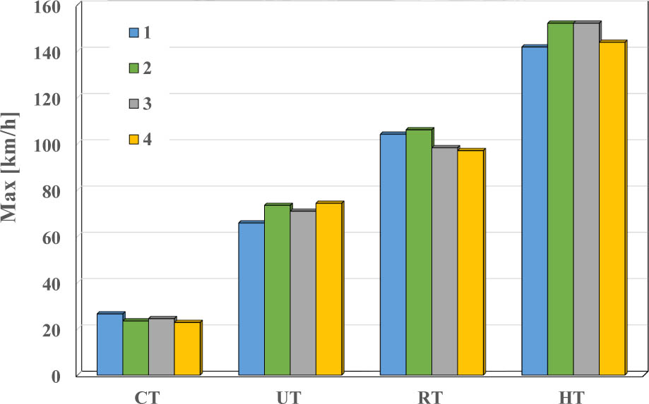
Figure 7.
Maximum value (Max) of the CT, UT, RT and HT velocity process representation
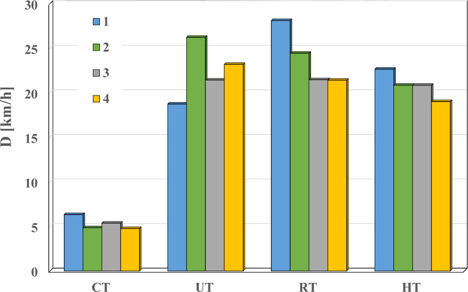
Figure 8.
Standard deviation (D) of the CT, UT, RT and HT velocity process representations
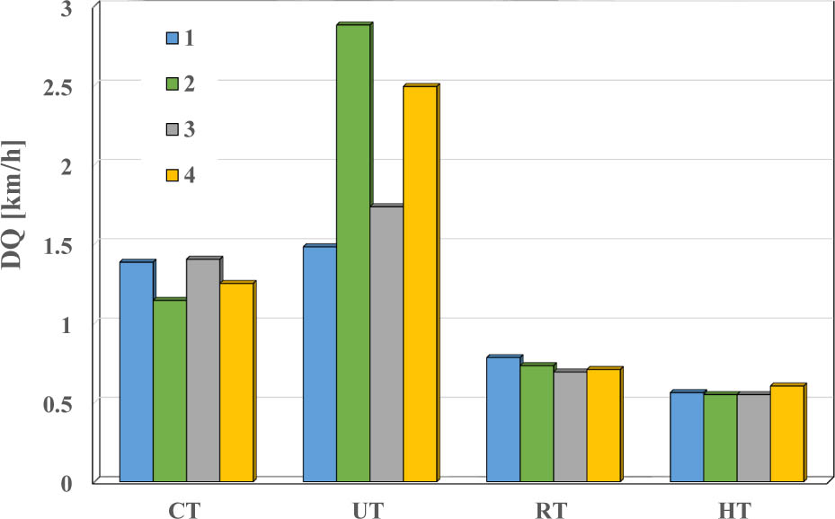
Figure 9.
Quartile deviation (DQ) of the CT, UT, RT and HT velocity process representations
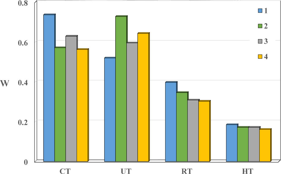
Figure 10.
Coefficient of variation (W) of the CT, UT, RT and HT velocity process representations
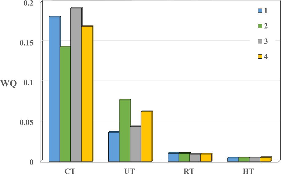
Figure 11.
Quartile coefficient of variation (WQ) of the CT, UT, RT and HT velocity process representations
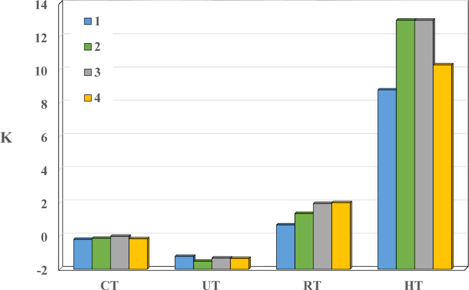
Figure 12.
Kurtosis (K) of the CT, UT, RT and HT velocity process representations
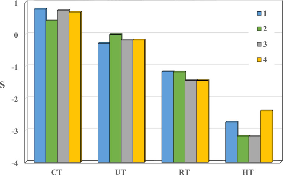
Figure 13.
Skewness (S) of the CT, UT, RT and HT velocity process representation
The average values for the individual velocity process representations CT, UT, RT and HT are similar. The same applies to the median and maximum values.
Figures 8–11 illustrate the distribution of key statistical parameters across process representations. The higher dispersion of standard deviation and coefficient of variation in urban driving reflects more dynamic velocity changes, which are known to increase fuel consumption and pollutant emissions. The low quartile coefficient of variation in HT confirms the stability of high-speed driving. The quartile coefficient of variation is definitely the smallest for the HT process, followed by the RT process.
The quartile coefficient of variation for the CT process is by far the largest. In the case of the coefficient of variation, the differences are not as large as in the case of the quartile coefficient of variation. The conclusions from the analysis of the coefficients of variation of the velocity processes clearly confirm that the strongest dynamic properties are characterized by the CT and UT processes, while the weakest by the HT process.
In the case of the CT test and especially the UT test, the distributions are platykurtic. For the RT and HT tests the distributions are leptokurtic. The greatest deviation from the normal distribution is for the HT test.
Only for the CT process the skewness is positive, i.e., the distribution is right-skewed. The remaining distributions are left-skewed, with the greatest deviation from the normal distribution for the HT test and the smallest for the UT test. In order to determine to what extent it is justified to recognize the recorded velocity curves as representations of the CT, UT, RT and HT velocity processes, the uniqueness of the zero-dimensional characteristics of the velocity process representation was examined. Uniqueness (U) of the test results was defined as the absolute value of the ratio of the standard deviation and the mean value:
The kurtosis and skewness values indicate that the velocity distributions deviate significantly from normality. Urban driving tends to produce platykurtic and right-skewed distributions, while fast-road driving produces leptokurtic and left-skewed distributions. These non-Gaussian characteristics highlight the need for stochastic modelling rather than parametric assumptions.
Figure 14 shows the uniqueness of the zero-dimensional characteristics of the CT, UT, RT and HT velocity processes. It was found that only in the case of skewness there is high non-repeatability.
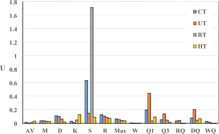
Figure 14.
The uniqueness (U) of the zero-dimensional characteristics of the CT, UT, RT and HT velocity process representations
Figure 15 shows the uniqueness of the mean value, maximum value and coefficient of variation of the CT, UT, RT and HT velocity process representations. It was found that the uniqueness of zero-dimensional characteristics of the CT, UT, RT and HT velocity process representations is small – in the case of the three characteristics considered, it is less than 0.07.
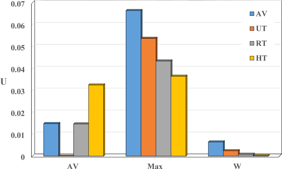
Figure 15.
The uniqueness (U) of the average value, maximum value and coefficient of variation of the CT, UT, RT and HT velocity process representations
Figures 16–19 show the probability density (g) for all process representations depending on the standardized velocity.
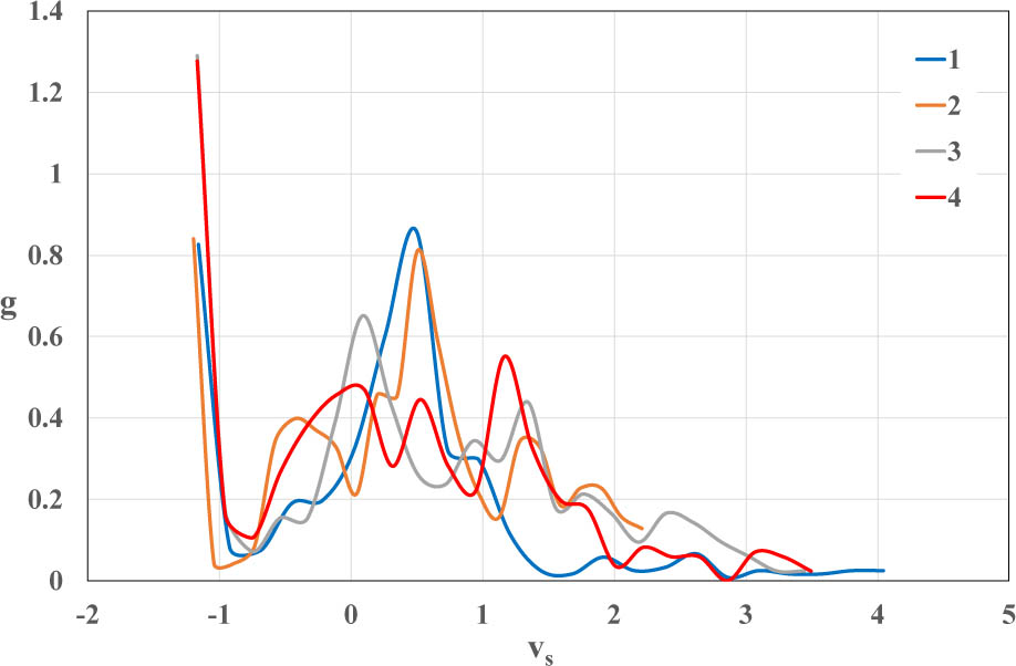
Figure 16.
Probability density (g) of the CT process representations depending on the standardized velocity (vs)
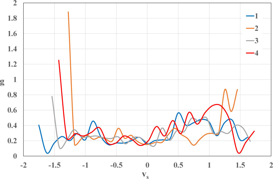
Figure 17.
Probability density (g) of the UT process representations depending on the standardized velocity (vs)
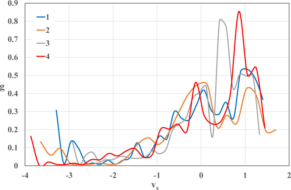
Figure 18.
Probability density (g) of the RT process representations depending on the standardized velocity (vs)
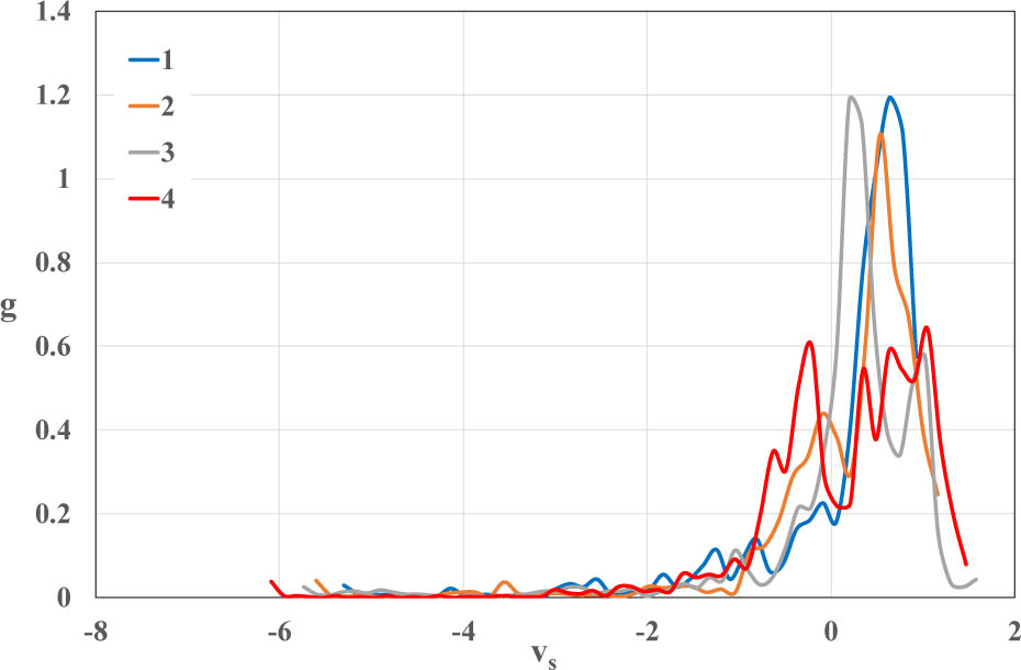
Figure 19.
Probability density (g) of the HT process representations depending on the standardized velocity (vs)
It was found that for urban driving (CT and UT) tests, the largest probability density is for small velocity values, while for extra-urban driving and fast road driving, the largest probability density is for large velocities. In most cases, the similarity of probability density for the representation of the same process is significant.
The compliance of the tested sets with the normal distribution was assessed. To test the hypotheses about the compliance of the studied sets with the normal distribution, the following hypotheses were used: Kolmogorov-Smirnov, Lilliefors and Shapiro-Wilk [Kolmogorov 1941; McClave, Sincich 2012; Shapiro et al. 1968; Smirnov 1948; Utts, Hackard 2014]. The probability of not rejecting the Kolmogorov-Smirnov, Lilliefors and Shapiro-Wilk hypotheses about the compatibility of the analysed sets with a normal distribution is less than 0.01. Therefore, it was concluded that there are no grounds for accepting the hypotheses about the compliance of the sets with the normal distribution.
The probability density functions show that urban driving is dominated by low-speed operation, while extra-urban and fast-road driving are dominated by high-speed operation. These differences directly influence emission formation mechanisms, as low-speed stop-and-go traffic increases transient engine loads, whereas high-speed driving increases aerodynamic drag and fuel consumption. Figures 20–23 show the power spectral density (G) of each velocity process representation, as well as the average value for all representations (AV), in the frequency domain (f). The power spectral density was determined using the fast Fourier transform and averaging the results with a simple moving average (SMA) filter [Bendat, Piersol 2010; Otnes, Enochson 1978; Ralston, Rabinowitz 2001].
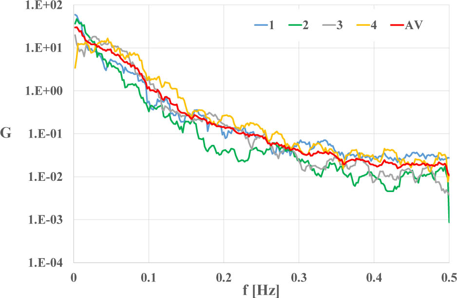
Figure 20.
Power spectral density of the CT process representations and the average value (AV) for all representations in the frequency domain (f)
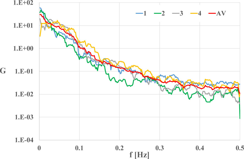
Figure 21.
Power spectral density of the UT process representations and the average value (AV) for all representations in the frequency domain (f)
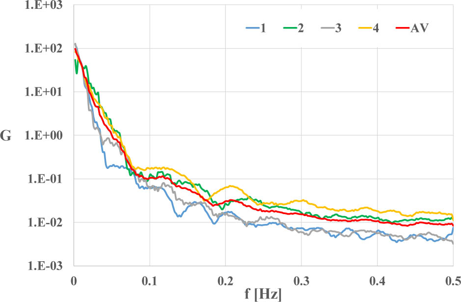
Figure 22.
Power spectral density of the RT process representations and the average value (AV) for all representations in the frequency domain (f)
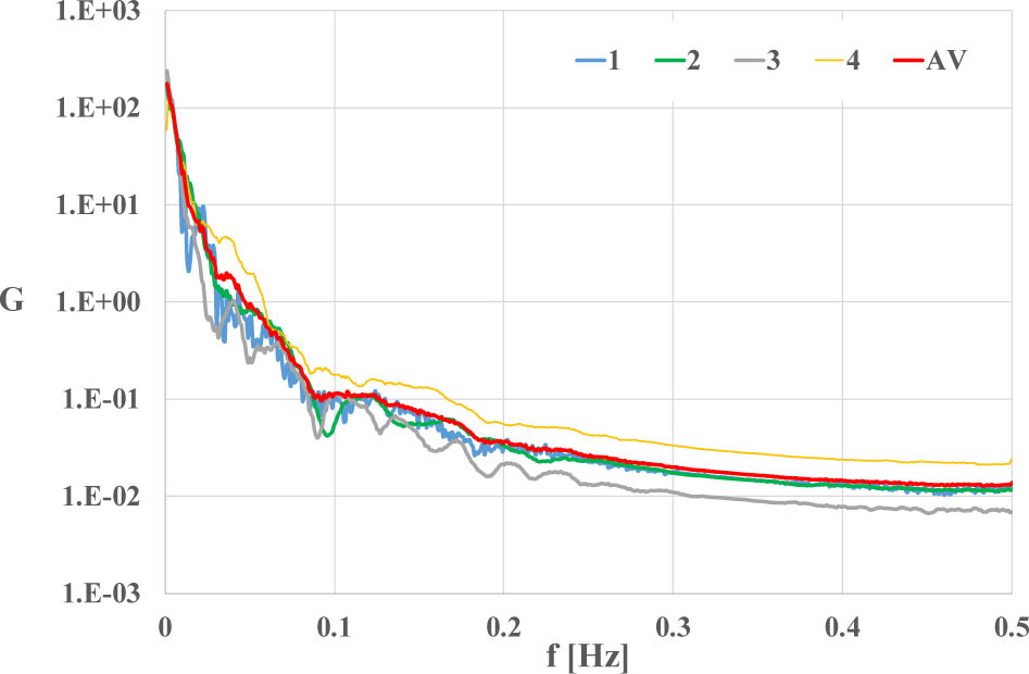
Figure 23.
Power spectral density of the HT process representations and the average value (AV) for all representations in the frequency domain (f)
The similarity of the power spectral density for the representations of the same process is significant.
Figure 24 shows a comparison of the power spectral density of the average value of the CT, UT, RT and HT process representations.
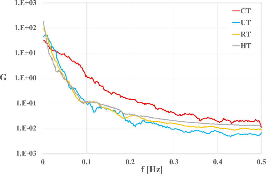
Figure 24.
The joint power spectral density of the CT, UT, RT and HT process representations in the frequency domain (f)
The value of power spectral density is the highest for the CT process, which confirms that this process is characterised by the strongest dynamic properties.
The power spectral density analyses reveal that urban driving contains strong low-frequency components, reflecting frequent accelerations and decelerations. These dynamic events are associated with increased emissions of nitrogen oxides, carbon dioxide and particulate matter. Fast-road driving shows lower spectral energy, indicating more stable velocity profiles. The comparison of power spectral density analysis across traffic conditions confirms that dynamic intensity is highest in urban environments.
CONCLUSION
Based on the research conducted, the following conclusions can be drawn:
There is a real possibility of determining the velocity tests for road vehicles in the form of stochastic processes. These tests can be represented as sets of velocity courses in repeatable conditions, typical of the characteristic conditions of vehicle use.
The study confirms that stochastic representations of driving velocity processes can be reliably constructed for characteristic traffic conditions: urban driving with congestion, urban driving without congestion, rural driving and fast-road driving. These representations constitute accurate simulations in the time domain and reflect the natural variability of real-world driving, which is essential for accurately assessing vehicle operational properties. The ability to model driving tests as stochastic processes provides a methodological alternative to deterministic driving cycles, offering improved realism and representativeness.
The justification for treating recorded velocity courses as representations of velocity processes was verified by analysing the uniqueness of zero-dimensional statistical characteristics.
The results show that the uniqueness (nonrepeatability) of key characteristics – mean value, maximum value and coefficient of variation is very small (below 0.07). This statistical stability indicates that the selected velocity courses form coherent sets and can be considered valid representations of the same underlying stochastic process. Such consistency is crucial for ensuring that the constructed stochastic tests are reliable and reproducible. Representative velocity processes were selected based on the similarity of their zero-dimensional statistical characteristics.
The research programme included analyses in three complementary domains: the time domain, the process value domain and the frequency domain. Time-domain analyses provided insight into the variability and dynamic behaviour of the velocity processes. The process value domain enabled the determination of probability density functions, revealing the distribution of velocity values under different traffic conditions. Frequency-domain analyses, based on power spectral density, allowed the identification of dominant dynamic components of the processes. Together, these domains offer a comprehensive description of the structure and properties of driving velocity processes.
The strongest dynamic properties were observed in urban driving processes, while the weakest were found in fast-road driving. This conclusion is supported by the analysis of both the coefficient of variation and the quartile coefficient of variation, as well as the power spectral density. Urban driving-especially under congestion-exhibits high variability, frequent accelerations and decelerations, and strong low-frequency components. In contrast, highway driving is characterised by more stable velocity profiles and lower dynamic intensity. These differences have direct implications for fuel consumption, engine operating states and pollutant emissions, which are known to increase under highly dynamic driving conditions.
The conformity of the studied sets to the normal distribution was assessed using the Kolmogorov-Smirnov, Lilliefors and Shapiro-Wilk tests.
For all analysed sets, the probability of not rejecting the hypothesis of normality was below 0.01. Therefore, there is no basis for accepting the hypothesis that the velocity processes follow a normal distribution. This finding confirms that real driving behaviour is inherently non-Gaussian, often skewed and heavy-tailed. As a result, classical parametric models assuming normality are insufficient for describing driving velocity processes, reinforcing the need for stochastic and non-parametric approaches.
Treating driving tests as stochastic processes of vehicle velocity enables the acquisition of extended knowledge about vehicle operational properties, especially under non-repeatable real-world conditions.
Stochastic modelling captures the natural variability of traffic, driver behaviour and environmental influences, which cannot be reproduced using deterministic driving cycles. This approach provides a more realistic basis for evaluating fuel consumption, pollutant emissions and dynamic engine behaviour. Consequently, stochastic driving tests can improve the accuracy of environmental assessments, emission inventories and simulation models, supporting both scientific research and practical applications in vehicle engineering and environmental policy.
The results demonstrate that stochastic velocity processes can support the development of more representative driving tests and improve the accuracy of emission modelling. Their ability to reflect real-world driving variability makes them valuable for environmental assessments, vehicle design and regulatory development. Future research should integrate stochastic velocity modelling with direct emission measurements, extend the approach to hybrid and electric vehicles, and explore region-specific stochastic driving patterns to support sustainable mobility planning.