
Table 1.
Screening performance of the fully connected neural network for the three types of coincidences
| K1 | T | R | S | NECR | RF (%) | SF (%) | |
|---|---|---|---|---|---|---|---|
| Training set | |||||||
| before primary screening | \ | 720 456 | 9 663 407 | 511 561 | 47 639.89 | 93.06 | 41.52 |
| after primary screening | \ | 709 268 | 567 957 | 484 086 | 285 617.42 | 44.47 | 40.57 |
| after secondary discrimination | −0.6 | 684 933 | 349 937 | 274 977 | 358 158.79 | 33.81 | 28.65 |
| Test set | |||||||
| before primary screening | \ | 89 947 | 1 216 793 | 64 059 | 5 902.01 | 93.12 | 41.59 |
| after primary screening | \ | 88 371 | 71 296 | 60 410 | 35 485.01 | 44.65 | 40.60 |
| after secondary discrimination | −0.6 | 84 479 | 43 237 | 34 518 | 43 990.17 | 33.85 | 29.01 |
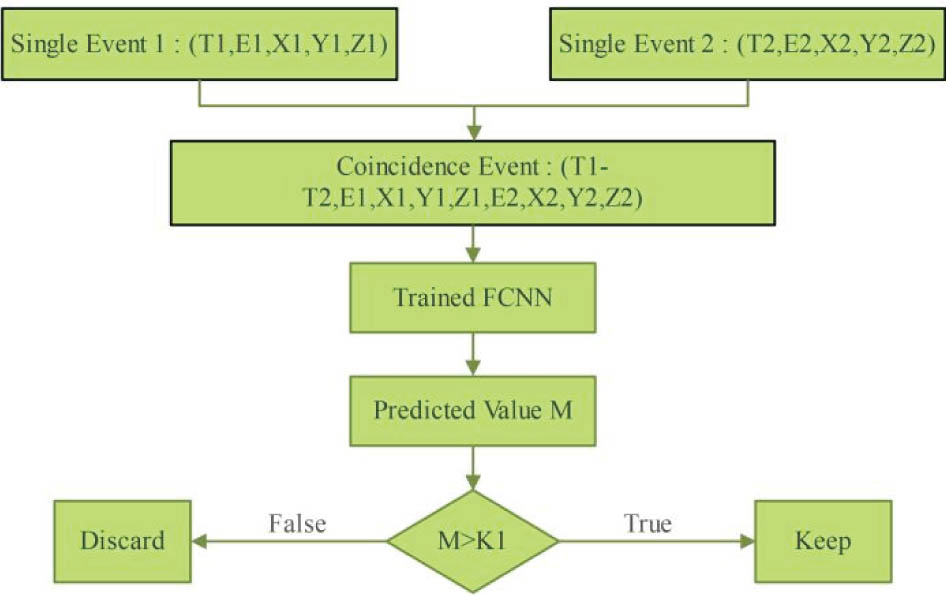
Fig. 1.
Schematic illustration of the true coincidence discrimination process.
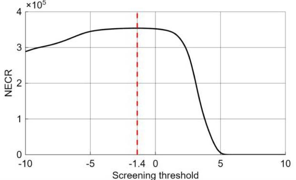
Fig. 2.
Variation of the noise equivalent counting rate (NECR) with the lower screening threshold.
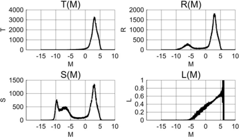
Fig. 3.
Schematic diagram of the distribution of predicted values for the three types of coincidences and the correction function.
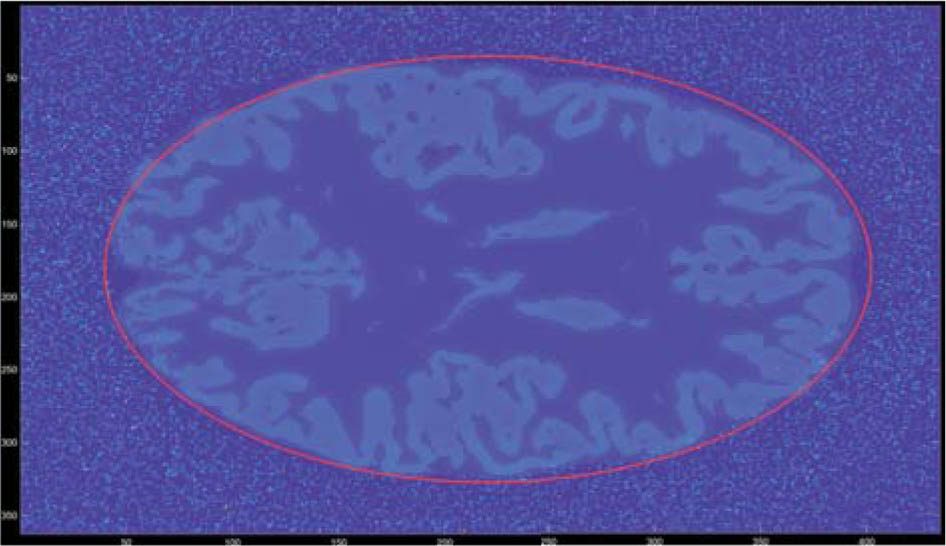
Fig. 4.
Example image of the annihilation point probability matrix after screening.
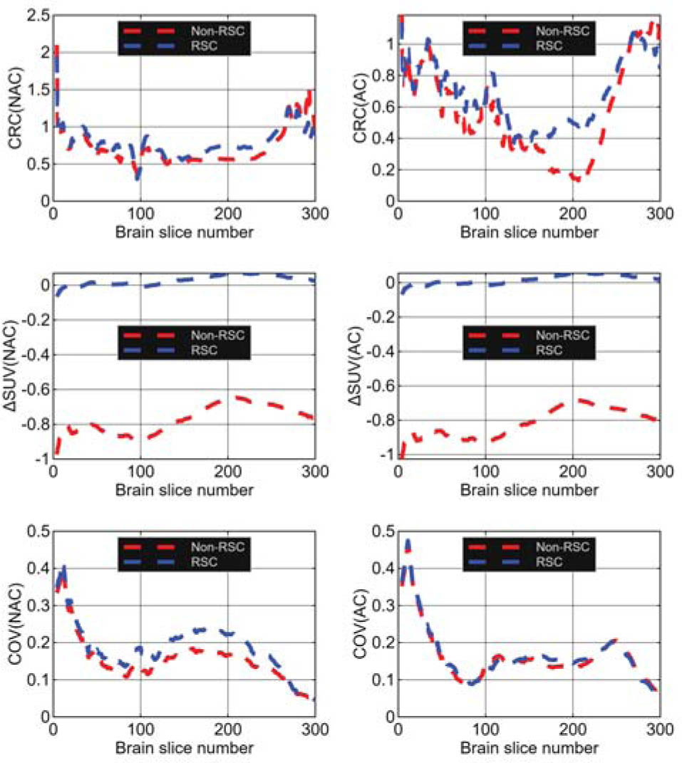
Fig. 5.
Comparison of the three metrics before and after attenuation correction.