
Introduction
Positron emission tomography (PET) is a medical imaging technique that utilizes radiotracers, such as 18-FDG, which undergo positron decay within the human brain. These positrons annihilate with electrons, emitting two γ-photons in opposite directions. Scintillation crystals detect these photons within a specific coincidence time window, and the detection times are recorded to calculate the annihilation point, enabling real-time brain imaging.
However, due to Compton scattering and the finite coincidence time window, three types of coincidence events are generated: true coincidences, scattered coincidences, and random coincidences. True coincidences constitute the core data for brain PET imaging, whereas scattered and random coincidences introduce significant noise into the reconstructed images.
For scattered coincidence correction, the most practical method currently is single scatter simulation (SSS), along with Monte Carlo (MC) scatter correction and deep learning-based sinogram scatter correction. The SSS method performs well in estimating single scattering events [2]. It requires an auxiliary step to estimate multiple scattering events, typically achieved by scaling the single scatter distribution estimate using tail-fitting techniques to match the measured data distribution, which includes multiple scattering events. This fitting process usually utilizes regions of the sinogram outside the emission source distribution. Depending on the imaging configuration and activity distribution, this process can be inaccurate, primarily because single and multiple scatter distributions have significantly different shapes, along with noise and other data inconsistencies between internal and external scatter distributions [2, 3]. Recent advancements involve dual scatter simulation (DSS) using only a subset of single scatter pairs, enabling absolute scaling and improved scatter correction results [4]. Regarding MC scatter correction, several studies have proposed MC-based scatter coincidence estimation methods [2, 5,6,7]. These methods have the potential to provide precise scatter estimates but require substantial computational resources, making them too time-consuming for routine clinical use. Although optimization techniques based on hybrid CPU/GPU architectures have been developed over the past decade to accelerate MC-based scatter estimation [8], the computational burden remains significant. As for deep learning (DL) scatter correction, after the training phase, DL offers the possibility of effectively solving complex and time-consuming tasks. Studies have explored the potential of using DL to directly perform scatter and attenuation correction in image space [9,10,11,12]. However, this method requires a large amount of training data and has been proven to fail when presented with images exhibiting variable quality and noise levels not encountered during training.
For random coincidence correction, the mainstream method is the singles counting rate technique. This involves introducing a time delay (longer than the coincidence time window) to measure the count rate of random coincidences without true coincidences, which is then subtracted from the total coincidence count [13, 14]. Alternatively, theoretical formulas are used for estimation and subsequent subtraction. The advantage of this method is that it improves the image signal-to-noise ratio (SNR), reduces quantitative errors, and yields more accurate SUV values [15]. However, the singles rate method is sensitive to dead time and detector efficiency, leading to higher errors. It also increases the count rate of coincidence events.
To address the issue of high computational resource consumption associated with correction methods such as SSS and singles counting rate estimation, this paper proposes a method utilizing a FCNN to rapidly filter coincidence data outside the brain region and perform rapid RSC within the brain slice region. Compared to SSS and delayed coincidence window methods, this approach omits complex correction procedures, thereby saving significant computational resources. The FCNN is a fundamental deep learning network with powerful feature learning capabilities, universality, and flexibility [16,17,18,19]. Given that the coincidence data required for brain PET imaging has relatively few features, it is highly suitable for rapidly establishing the relationship between coincidence data information and event types.
This paper first introduces the basic imaging principle of brain PET technology. A polyhedral brain PET detector model was constructed based on GATE. Subsequently, the relationship between coincidence data information and event types was investigated using FCNN. Finally, a method based on FCNN for rapid filtering of coincidence data outside the brain region and RSC within the brain slice region is proposed.
GATE simulation
Simulation model construction
Regarding the detector model, polyhedral brain PET offers higher detection efficiency and geometric adaptability compared to conventional ring-shaped brain PET, resulting in the processing of more data within the same timeframe [20,21,22]. To investigate fast random and scatter correction for polyhedral brain PET, a polyhedral brain PET detector model based on the great rhombicuboctahedron was constructed using the GATE simulation platform. The scintillation crystals selected were LYSO, with dimensions of 4 mm × 4 mm × 20 mm, separated by a 0.2 mm gap. The selection of 4 mm × 4 mm × 20 mm LYSO crystals with a 0.2 mm gap is based on established designs for high-resolution PET scanners [23]. This configuration offers an optimal balance between spatial resolution, detection efficiency, and depth of interaction (DOI) effects [20].
For the phantom model, to closely mimic the actual human brain structure, this study utilized a 3D brain phantom derived from 11 human brains developed by Aubert-Broche et al. [24]. This phantom features strict delineations of brain regions and material assignments, allowing for the classification into 12 distinct tissue regions based on pixel values [24]. The corresponding tissue regions and pixel values are listed in Table 1. Each brain phantom model is divided into 362 slices along the axial direction, with each slice measuring 362 pixels × 434 pixels. The voxel size is 0.5 mm × 0.5 mm × 0.5 mm.
Table 1.
Screening performance of the fully connected neural network for the three types of coincidences
| K1 | T | R | S | NECR | RF (%) | SF (%) | |
|---|---|---|---|---|---|---|---|
| Training set | |||||||
| before primary screening | \ | 720 456 | 9 663 407 | 511 561 | 47 639.89 | 93.06 | 41.52 |
| after primary screening | \ | 709 268 | 567 957 | 484 086 | 285 617.42 | 44.47 | 40.57 |
| after secondary discrimination | −0.6 | 684 933 | 349 937 | 274 977 | 358 158.79 | 33.81 | 28.65 |
| Test set | |||||||
| before primary screening | \ | 89 947 | 1 216 793 | 64 059 | 5 902.01 | 93.12 | 41.59 |
| after primary screening | \ | 88 371 | 71 296 | 60 410 | 35 485.01 | 44.65 | 40.60 |
| after secondary discrimination | −0.6 | 84 479 | 43 237 | 34 518 | 43 990.17 | 33.85 | 29.01 |
Regarding the source model, to construct a high-fidelity digital source, this study employed an anatomy-constrained physiological modeling approach. Taking into account the spatial continuity of tracer uptake and the complexity of microstructures in real biological tissues, we convolved the high-resolution anatomical phantom with a point spread function (PSF). This process effectively simulates the biological partial volume effect at tissue interfaces, generating a radiotracer activity distribution map with natural gradient transitions, thereby avoiding non-physiological artifacts inherent in ideal step-function models [25, 26]. A linear mapping relationship between pixel values and activity was established. The radiation source consisted of γ-photons with an energy of 511 keV, emitted in opposite directions.
In terms of simulation parameters, the Monte Carlo simulation was configured to emulate a modern clinical TOF-PET scanner. The detector time resolution was set to 300 ps to represent state-of-the-art systems. An energy resolution of 15% at 511 keV was assumed. Data were acquired within a 400–600 keV energy window to reject scattered events. The system dead time was modeled as 110 ns in non-paralyzable mode, and a 5 ns coincidence time window was applied, consistent with established simulation protocols [27].
Simulation procedure
Based on the phantom and source parameters set in the previous section, eleven simulations were conducted. During these simulations, only the brain phantom and source models were varied, while all other settings remained constant. The centers of the phantom, source, and the polyhedral brain PET detector were all aligned at the coordinate origin. When γ-photons emitted from the source interacted with the scintillators, the simulation recorded eight specific pieces of information for each photon: (event ID, time T, deposited energy E, interaction coordinates (X, Y, Z), Compton scattering ID, Rayleigh scattering ID).
Correction methods and evaluation metrics
Neural network architecture
Based on the simulation results, coincidence recombination was performed on the recorded events using a coincidence time window to obtain the initial coincidence events. These coincidence events were subsequently classified into three categories based on Compton scattering occurrence and other information, and corresponding labels were assigned. For the input layer, assuming a coincidence event includes the following information: response event 1 consists of response time T1, response energy E1, response coordinates (X1, Y1, Z1), and response event 2 consists of response time T2, response energy E2, response coordinates (X2, Y2, Z2). Thus, the input layer for a single coincidence event is represented as a 1 × 9 vector (T1–T2, E1, X1, Y1, Z1, E2, X2, Y2, Z2). The output layer is a 1 × 1 vector, where a value of 10 indicates a true coincidence, 0 indicates a scattered coincidence, and −10 indicates a random coincidence.
To enhance the quality of coincidence data within the training set, a two-stage true coincidence discrimination process was implemented. The first stage involved eliminating coincidence data where the annihilation point was outside a specified cubic volume, determined by calculating the annihilation point for each event. Specifically, the ten digital brain phantoms used for training, testing, and validation were all located within a cubic space defined by X ranging from −90.5 mm to 90.5 mm, Y ranging from −108.5 mm to 108.5 mm, and Z ranging from −90.5 mm to 90.5 mm.
The FCNN training served as the second stage of true coincidence discrimination. For dataset configuration, coincidence data processed from the first eight digital brain simulations were used as the training set, while data from the ninth and tenth simulations were used as the validation set and test set, respectively.
The FCNN was implemented in MATLAB R2025a. To optimize the model architecture and training parameters – including the number of fully connected layers, neurons per layer, initial learning rate, and L2 regularization coefficient – Bayesian optimization was utilized [28]. During this process, 5-fold cross-validation was embedded within every optimization iteration, providing the evaluation feedback necessary for the algorithm to iteratively update and select the optimal hyperparameters [29].
The Bayesian optimization process ran for 59 iterations, at which point the mean squared error (MSE) had converged. The final architecture of the FCNN consists of an input layer, five hidden layers, and an output layer. The input layer accepts a 1 × 9 vector, and the output layer produces a 1 × 1 vector. The number of neurons in the five hidden layers are 511, 217, 126, 18, and 1, respectively. A ReLU activation function is applied between each hidden layer. The optimized initial learning rate is 0.0016658, and the L2 regularization coefficient is 0.000024817.
For the K-fold cross-validation, the final result yielded an MSE of 54.313 ± 0.153.
True coincidence discrimination and random/scatter correction
True coincidence discrimination
As illustrated in Fig. 1, based on the trained network framework, the input layer of the training set is first imported for prediction, yielding a corresponding predicted value M for each coincidence event via FCNN. A lower threshold K is then set to filter coincidence events where M > K, which are presumed to be true coincidences. By comparing these predictions with the actual output layer of the training set and incrementally increasing K, the value K1 is determined when the NECR reaches its maximum. Subsequently, this optimal threshold K1 is applied to the test set to obtain the final predicted NECR.
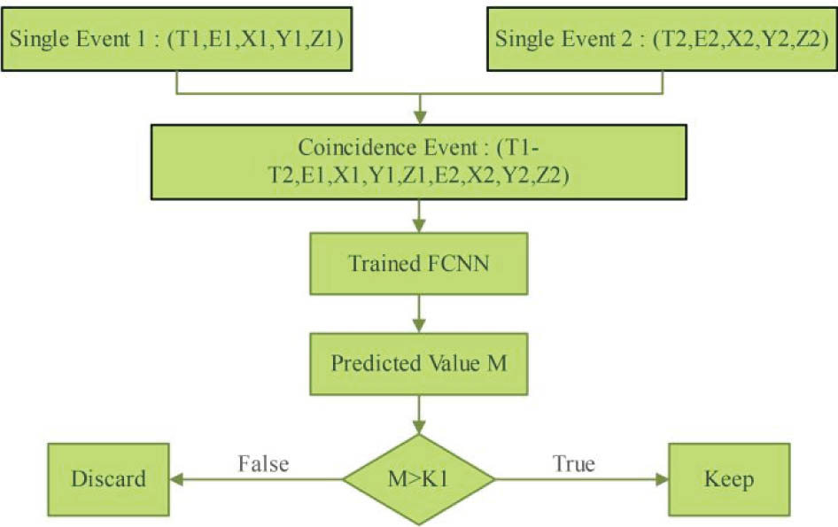
Fig. 1.
Schematic illustration of the true coincidence discrimination process.
Random and scatter coincidence correction method
Based on the training results, a correction method for RSC is proposed. The eleventh digital brain phantom is selected to evaluate the training performance. The specific methodology is as follows.
In time-of-flight positron emission tomography (TOF-PET), for a specific line of response (LOR), the system matrix element aij can be decomposed into the product of a geometric component Gij and a TOF kernel function Kij (Δt) [30,31,32]:
Since the types and predicted values M of each coincidence event in the training set are known, the distribution functions of true coincidences, scatter coincidences, and random coincidences with respect to the predicted value M can be denoted as T(M), S(M), and R(M), respectively. The correction function is defined as L(M), expressed by the following equation:
For an unknown coincidence event, its predicted value M can be obtained using the trained FCNN. By inputting this M into the correction curve function L(M), the contribution value L of the true coincidence for this event is derived. Based on this true coincidence contribution value L, RSC for the brain PET image can be performed. For a specific LOR, incorporating Eq. (2), it can be expressed as follows:
To evaluate the training performance, this study employed the single-slice rebinning (SSRB) method to reconstruct images from the coincidence data using the filtered back projection (FBP) algorithm [33, 34]. For 2D voxel assignment along the LOR, a Gaussian kernel function was utilized to distribute values around the annihilation point along the LOR, with a standard deviation of 5 mm. The reconstruction matrix was set to 362 × 434 × 362, with a voxel size of 0.5 mm. The FBP reconstruction matrix image without RSC is denoted as IMG1. The FBP reconstruction matrix image with RSC applied is denoted as IMG2. Furthermore, the FBP reconstruction matrix image generated solely from true coincidence data is denoted as IMG3.
To comprehensively evaluate the performance of the proposed FCNN-based RSC method, both attenuation-corrected (AC) and non-attenuation-corrected (NAC) reconstructions were performed.
For the AC scenario, an analytical attenuation correction was applied. Based on the known anatomical structure and material composition of the digital brain phantom, a theoretical attenuation map (μ-map) was generated. The attenuation factors were then calculated analytically via ray-tracing through this map and applied to the sinogram data prior to reconstruction [35].
It should be noted that the attenuation correction was performed as a standard pre-processing step and was independent of the FCNN model, which focused solely on random and scatter coincidence discrimination.
Evaluation metrics
Evaluation metrics for true coincidence discrimination
To evaluate the performance of true coincidence discrimination, this study adopted the noise equivalent count rate (NECR), scatter fraction (SF), and random fraction (RF). The NECR is primarily used to assess the SNR within the imaging data; a higher NECR indicates lower noise levels in the reconstructed image. The SF measures the proportion of scattered coincidences in the imaging data; a lower SF indicates reduced scatter noise. Similarly, the RF measures the proportion of random coincidences; a lower RF indicates reduced random noise [36, 37].
The equation defines T as the number of true coincidences, S as the number of scattered coincidences, and R as the number of random coincidences.
Evaluation metrics for random and scatter coincidence correction
To comprehensively evaluate the performance of random and scatter coincidence correction (RSC) in PET imaging, three key quantitative metrics were employed: the contrast recovery coefficient (CRC), the signal-to-noise ratio (SNR), and the contrast-to-noise ratio (CNR). These metrics collectively assess the accuracy of contrast representation, image clarity, and lesion detectability [38,39,40].
CRC. The CRC primarily measures the accuracy of contrast recovery in the reconstructed image, reflecting the system's ability to restore the true radioactivity concentration contrast. It is defined as the ratio of the measured contrast in the image to the actual physical contrast. A CRC value closer to 1 indicates superior correction for random and scatter coincidences, implying higher image fidelity and quantitative accuracy.
where: SUVsphere(mean) – the mean standardized uptake value within the region of interest; SUVbackground(mean) – the mean standardized uptake value within the background region; Activitysphere – the true radioactivity concentration in the sphere/lesion region; Activitybackground – the true radioactivity concentration in the background region.SNR. The SNR reflects the overall clarity of the image by comparing the strength of the desired signal to the level of background noise. A higher SNR indicates a clearer image with less noise interference, which is essential for visual interpretation. In this context, it is calculated based on the maximum signal intensity within the lesion relative to the noise level in a homogeneous reference region.
where: SUVlesion(max) – the maximum standardized uptake value within the lesion/ROI; σbackground – the standard deviation of the signal within the background region.CNR. The CNR evaluates the distinguishability of the target region from the background relative to the noise level. It combines both the contrast difference and the noise characteristics, serving as a critical indicator for assessing lesion detectability. A higher CNR ensures that the contrast between different tissues is significantly greater than the background noise, facilitating accurate diagnosis.
where: μlesion – the mean signal intensity within the lesion; μbackground – the mean signal intensity within the background region; σlesion – the standard deviation of the signal within the lesion (representing noise); σbackground – the standard deviation of the signal within the background region.Results and analysis
True coincidence discrimination
The GATE simulation required 354 hours, and the deep learning model completed 1 720 000 iterations. The training results demonstrate high computational efficiency: when predicting 1 761 742 coincidence events, the fully connected neural network required only 9.733550 seconds, averaging 5.52495768 × 10⁻⁶ seconds per event. This indicates the method significantly conserves computational resources and enables rapid prediction for subsequent correction processing.
Figure 2 illustrates the variation of NECR with the lower screening threshold K1. As K1 increases, the NECR gradually rises, reaching a maximum of 353 987.40 when K1 is approximately −0.6. This phenomenon is explained by Fig. 3, which depicts the distribution of predicted values for the three coincidence types and the correction function L(M). The primary reason for setting a lower threshold is that scatter coincidences S(M) and random coincidences R(M) have significant proportions when M< −0.6, whereas L(M) is primarily distributed for M> −0.6. This allows for the easy removal of scatter and random coincidences with predicted values below −0.6. However, in the region where M> −0.6, many random and scatter coincidences remain, as their predicted values largely overlap with those of true coincidences, making them difficult to distinguish. Therefore, a secondary discrimination process was implemented.
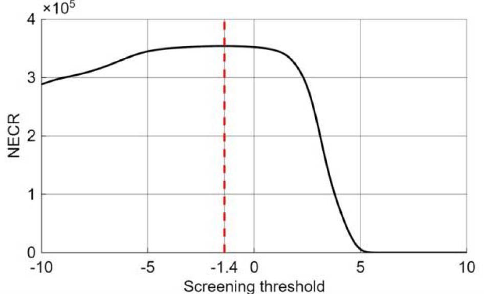
Fig. 2.
Variation of the noise equivalent counting rate (NECR) with the lower screening threshold.
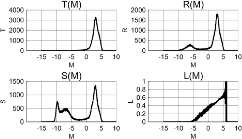
Fig. 3.
Schematic diagram of the distribution of predicted values for the three types of coincidences and the correction function.
As shown in Table 1, after secondary discrimination, the NECR of the test set increased from 35 485.01 to 43 990.17. The random fraction (RF) decreased from 44.65% to 33.85%, and the scatter fraction (SF) decreased from 40.60% to 29.01%. Meanwhile, 95.60% of the true coincidences were retained, preserving the core imaging data while significantly reducing random coincidences and thereby minimizing imaging noise interference.
Figure 4 displays the annihilation point probability matrix generated from the filtered coincidence data (predicted values M< −0.6) for brain slice 181. The image shows that the filtered annihilation points are predominantly distributed outside the brain slice (outside the red box), with almost no removal of scatter or random coincidences occurring within the brain slice (inside the red box). This demonstrates that the method effectively removes invalid coincidence data outside the brain region, enhancing the quality of the coincidence data for subsequent imaging processing.
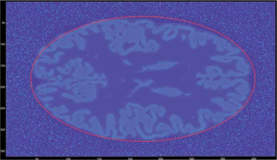
Fig. 4.
Example image of the annihilation point probability matrix after screening.
Random and scatter coincidence correction
Given the overlap of predicted values for true, random, and scatter coincidences when M> −0.6, this paper applied Eq. (3) to perform RSC on this subset of data. As shown in Fig. 5, the CRC, SNR, and CNR were subsequently calculated.
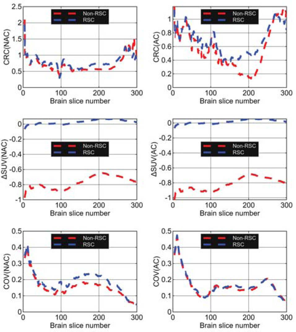
Fig. 5.
Comparison of the three metrics before and after attenuation correction.
The experimental results demonstrate that the proposed RSC method significantly optimizes image quality when synergistically combined with AC. Under AC conditions, the application of RSC elevated the CRC from 0.946 to 0.969, boosted the SNR substantially from 10.24 to 19.13, and improved the CNR from 0.402 to 0.496 compared to the non-RSC baseline. This confirms the method's effectiveness in purifying the signal through accurate modeling and subtraction of scatter and random events, where AC recovers true count magnitude while RSC removes spurious events, resulting in a synergistic enhancement of contrast recovery and noise suppression.
Conversely, under the NAC condition, the differential impact of RSC on separate metrics necessitates a nuanced explanation grounded in the physical definitions of each parameter. Specifically, the CRC saw a slight increase from 0.945 to 0.971; this marked improvement is a direct consequence of RSC's ability to restore true concentration differences by removing spurious signals that mask true lesions and blur image details, making CRC the most sensitive metric to signal purity. In stark contrast, the SNR deteriorated from 11.53 to 9.73 because the removal of scatter and random components leads to a net loss of total counts without AC compensation, thereby increasing statistical noise according to Poisson statistics (noise ∝ 1/√N). Consequently, the CNR exhibited an intermediate behavior, decreasing slightly from 0.569 to 0.521, as it represents the composite effect of competing factors where the gain in contrast is offset by the increase in noise.
Therefore, the distinct performance trends observed under NAC do not indicate algorithmic failure but rather reflect the inherent trade-off between physical accuracy and statistical quality, further underscoring that the proposed RSC method is optimally deployed in conjunction with AC.
Conclusion
This study primarily designed a polyhedral brain PET detector based on the great rhombicuboctahedron using Geant4. This detector was employed to simulate the detection of eleven brain phantoms, generating three types of coincidence events. The research focused on methods for the rapid filtering of coincidence data outside the brain region and fast random and scatter coincidence correction within the brain region. By utilizing the inherent time difference, energy, and position information of coincidences as the input layer, a fully connected neural network was trained to establish the mapping relationship. The output layer's predicted values were then used to discriminate true coincidences and perform random and scatter correction.
The results demonstrate that the fully connected neural network can effectively filter coincidence data outside the brain slices and rapidly perform random and scatter correction within the brain slices. After correction, the metrics showed significant improvement: quantitative evaluation demonstrates that the RSC method significantly enhances image quality when combined with AC, improving the CRC from 0.946 to 0.969, SNR from 10.24 to 19.13, and CNR from 0.402 to 0.496. Conversely, under NAC conditions, RSC improves CRC (0.945 to 0.971) but reduces SNR (11.53 to 9.73) and CNR (0.569 to 0.521), indicating a trade-off between signal purity and statistical noise. The radioactivity concentration in the gray matter regions was accurately recovered, and the method required relatively low computational resources, indicating strong potential for practical application.
Acknowledgments
This work received no specific grant from any funding agency. There are no individuals or institutions to acknowledge.